
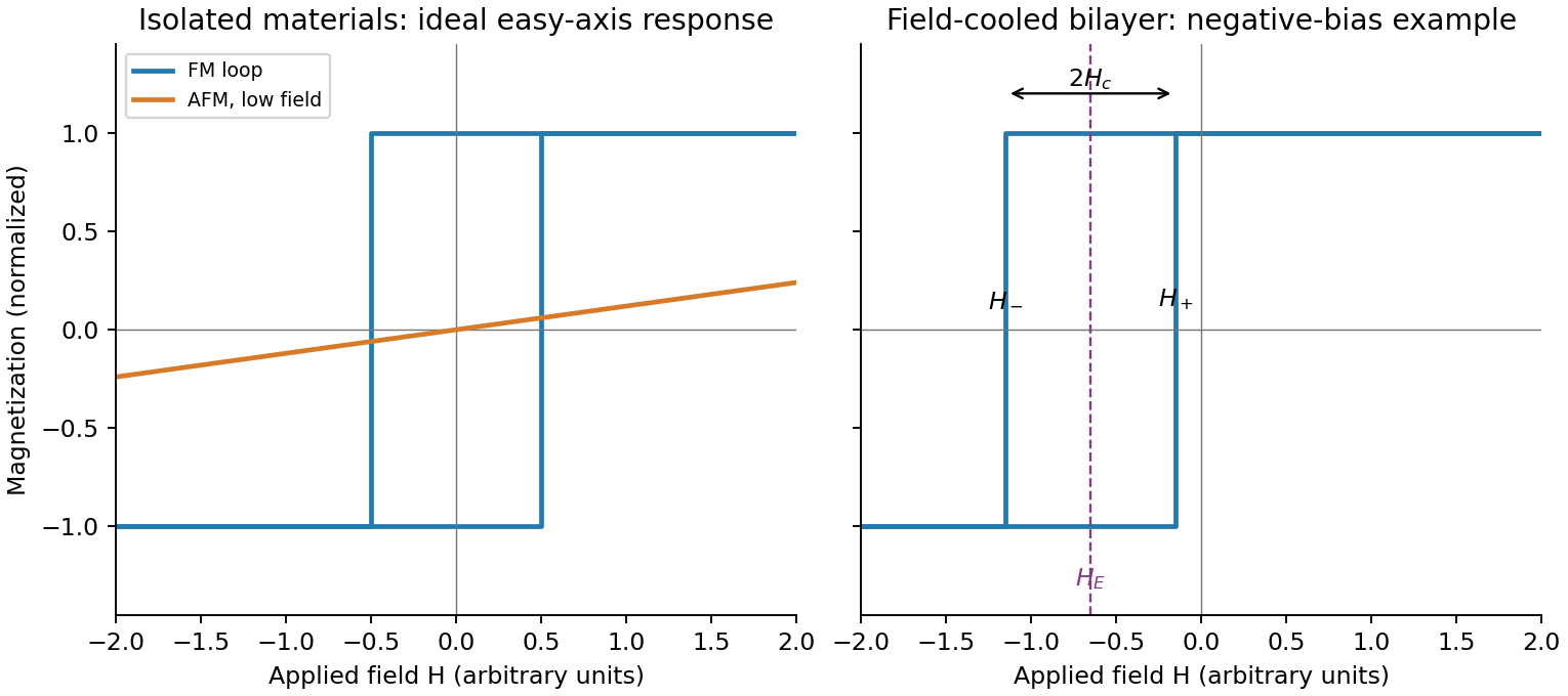
Write the descending and ascending switching fields as and . The exchange bias loop centre and magnetic coercivity half-width areWith exchange bias, a field-cooled bilayer has , often a shift opposite to the cooling field for the conventional negative-bias case shown in the diagram. The sign is not universal; it depends on interfacial coupling and preparation. A simple rigid-pinning estimate is .
Cooling farther below the blocking range usually strengthens antiferromagnetic anisotropy and suppresses thermal relaxation, so the magnitude of the shift and often the coercive width grow. Close to or above the blocking temperature the shift disappears; the blocking temperature can be below . Repeated cycling can rearrange interfacial spins and reduce the bias, and the two reversal branches can acquire different shapes. Thus increasing low-temperature asymmetry is a common tendency, not a guaranteed monotonic law for every interface.
Heat the bilayer into a window , apply an in-plane magnetic field sufficient to align the ferromagnet, and cool through the antiferromagnet's ordering/blocking range while retaining the field. The ferromagnet supplies a preferred interfacial spin direction as the antiferromagnet orders. Sufficient antiferromagnetic anisotropy then pins part of the interfacial spin configuration, producing unidirectional magnetic anisotropy rather than merely uniaxial magnetic anisotropy in the ferromagnet.
Measure a full major hysteresis loop after removing the cooling field, and compare with the isolated ferromagnet, a zero-field-cooled bilayer and the result of reversing the cooling-field direction. Those controls separate a true loop-centre shift from a changed coercive width, minor-loop artefacts or trapped applied field. The effect requires appropriate interfacial exchange and stable pinning; an ideally compensated or freely rotating interface need not produce a large bias. Exchange anisotropy in coupled ferromagnetic/antiferromagnetic material was demonstrated in the classic experiment below.[ref]
New Magnetic Anisotropy by W. H. Meiklejohn and C. P. Bean. Physical Review 102 (1956), pp. 1413–1414
For an isolated easy-axis ferromagnet undergoing coherent reversal, the ideal low-temperature loop is approximately rectangular, switching between at . It has remanent Magnetization and a large response near switching. An ideal compensated antiferromagnet has essentially no remanence and a small, approximately reversible linear net Magnetization at fields far below its exchange/spin-flop scales. Strong antiferromagnetic exchange makes substantial canting costly, so its low-field magnetic susceptibility is small relative to the ferromagnet's unsaturated switching response.
This comparison does not say the ferromagnet has a larger differential slope at every field: on its saturated branches can also be small. Nor does it rule out spin-flop transitions at much larger fields, outside the sketched range. The original plot uses arbitrary normalized scales.
The addition energy has both charging and orbital terms,The larger diamonds indicate quantum dot shell closure after 2, 6 and 12 electrons. A two-dimensional isotropic harmonic oscillator confinement, , explains that sequence: shell has orbital states and capacity after spin degeneracy. The cumulative capacities are . Within a degenerate shell, the extra orbital term vanishes to this approximation; crossing a shell boundary costs an extra .
The gate capacitance lever arm is . Large and small gate widths differ by , so . Equivalently the tip energies differ by . Confinement anisotropy, exchange and disorder would split the ideal degeneracies; the diagram supports approximate shell symmetry rather than proving a perfectly parabolic potential.
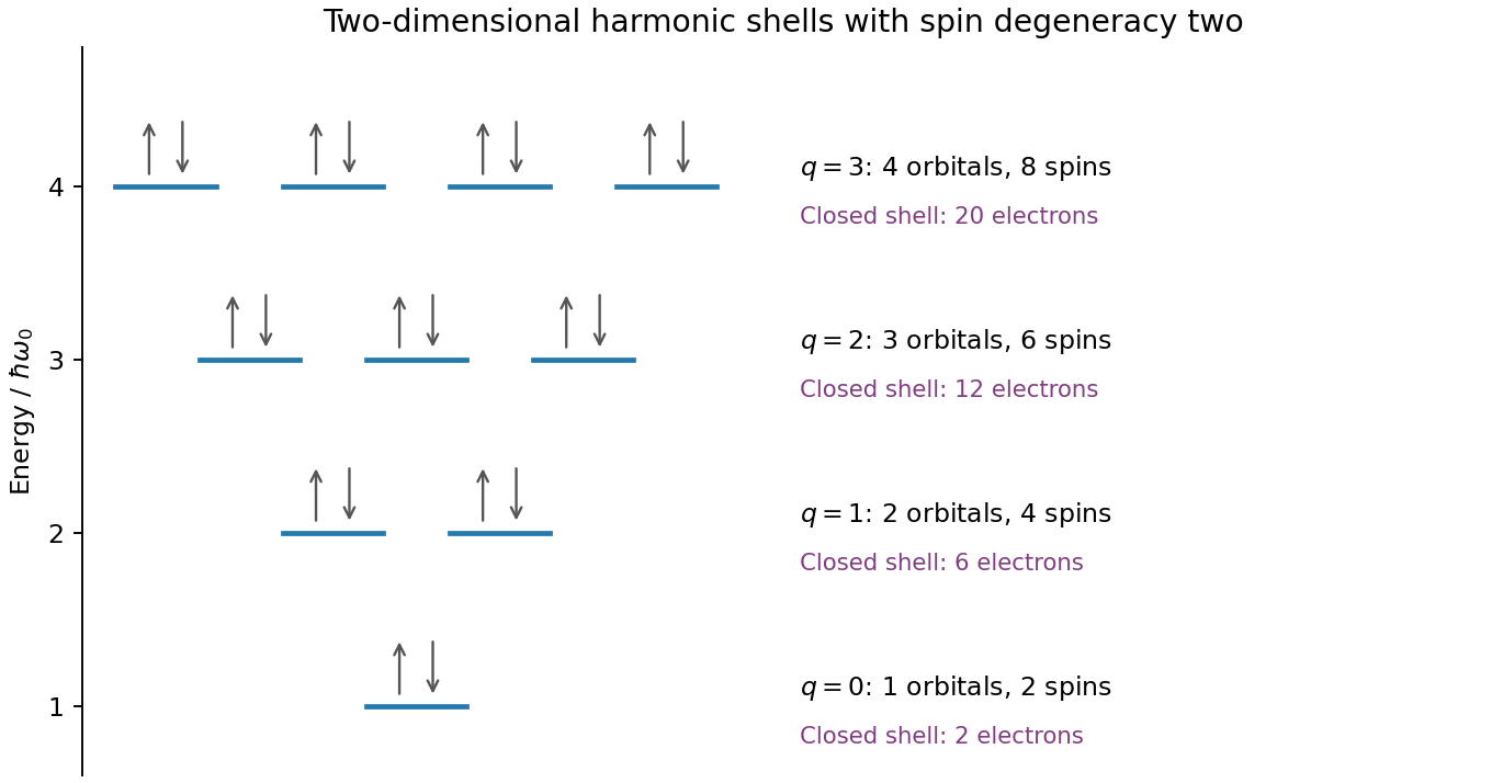
Original spin-degenerate two-dimensional oscillator shell capacities and closed-shell electron counts
. Details. Assume the usual one-lead-biased measurement, with drain grounded and the gate referred to that ground; the printed map does not separately specify the wiring. This assumption is needed to assign individual source/drain capacitances. In this Coulomb diamond capacitance extraction, the smaller zero-bias gate intervals are 5 mV wide. In the constant interaction model with no orbital gap between those additions,An upper diamond tip lies at gate 123.75 mV between the zero-bias vertices 120 and 125 mV and at bias 2.50 mV. Its positive and negative edge slopes are therefore and . Reservoir alignment givesThe gate capacitance is not negligible in the second denominator. ConsequentlyThe consistency check is , matching the smaller tip's bias energy. The conventional electrostatic charging energy is 1.25 meV; it is half the charging energy contribution to the addition energy. A different applied-bias convention changes the slope formulas, so the convention must accompany the extraction.
The map shows Coulomb blockade with discrete single-electron charging: low-current diamonds separate charge-stable regions from finite-bias transport windows. A small conducting island or quantum dot must be tunnel-coupled to source and drain, with a gate shifting its electrochemical potential. Charging prevents sequential transport until an island addition/removal energy enters the bias voltage window.
The tunnel resistances should substantially exceed the resistance quantum , preventing charge fluctuations from washing out integer island occupancy, while still permitting a measurable current. Temperature and tunnel broadening must be small compared with the addition-energy scale. Here the smaller diamonds imply , so , or ; resolving the inferred 1 meV orbital structure requires the stricter scale . Stray capacitance and unintended multiple islands can complicate this simple interpretation.
In terms of diameter , the model isThus melting temperature rises toward the bulk value as diameter increases, with a depression proportional to . The analytic sketch below includes the calculated point. It deliberately does not extrapolate the continuum expression down to a zero or negative melting temperature.
Facet-dependent energies, non-spherical shapes, size-dependent interfacial energies and latent heat, structural changes or magic cluster sizes can modify the trend. Premelting can broaden the transition. A substrate or encapsulating matrix changes interface energetics and can stabilize or destabilize the solid. Ligands, impurities, strain, particle size distributions, coalescence during heating and nonequilibrium temperature/beam effects can shift the measured transition. These possibilities motivate separate thermal, structural and size controls rather than a fit to diameter alone.
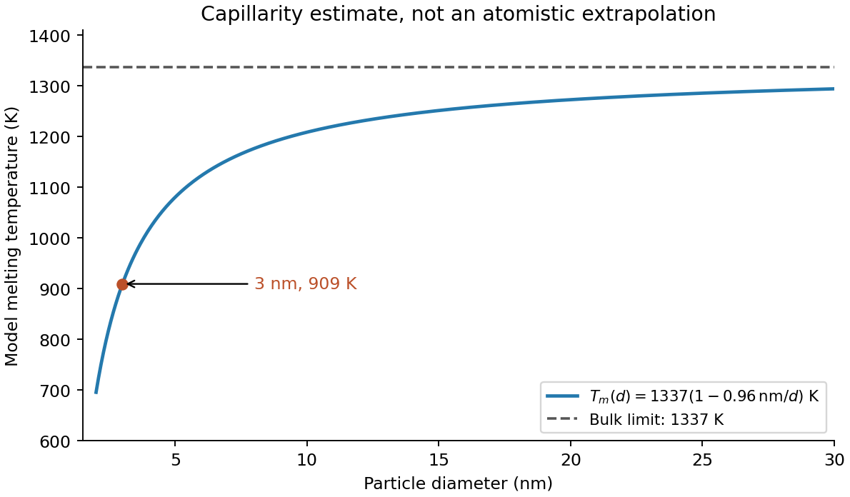
The radius is half the diameter, , and the latent heat density is . HenceUsing the diameter directly in the radius formula would underestimate the depression by a factor of two. The result is the stipulated continuum-model estimate; at only a few nanometres atomistic structure and support effects can matter substantially.
Let be the liquid-minus-solid free energy density at the same temperature. Near the bulk coexistence temperature , linearization givesFor a sphere, an interface displacement changes area and volume with . Equality of the bulk driving force and the capillary cost at a curved solid–liquid interface therefore gives . Equivalently, differentiating gives the same stationary radius. Combining the expressions yieldsThis form of the Gibbs-Thomson effect assumes isotropic interfacial energy, a spherical interface, bulk-like latent heat per volume and a near-coexistence free energy expansion. More detailed free-particle models must distinguish solid–vapor, liquid–vapor and solid–liquid energies.
Prepare size-characterized gold-particle ensembles, heat them on a calibrated in-situ electron diffraction stage, and follow the loss of sharp fcc diffraction features and appearance of liquid-like diffuse scattering. Measure the particle size distribution rather than treating a polydisperse ensemble as one diameter. Temperature-dependent weakening of a diffraction peak alone is insufficient: thermal vibrations, particle motion, coalescence, evaporation and beam damage can also reduce intensity. Low-dose repeats, heating/cooling runs, size checks before and after heating, a bulk-like reference and support-dependent controls help distinguish melting from those effects. Electron diffraction measurements on gold particles down to about 2 nm are a classic demonstration.[ref]
Size effect on the melting temperature of gold particles by Ph. Buffat and J-P. Borel. Physical Review A 13 (1976), pp. 2287–2298, abstract: scanning diffraction and size-distribution analysis
The physical origin is the large interface contribution to free energy at small radius. A curved solid–liquid interface raises the solid's thermodynamic equilibrium chemical potential relative to the flat-interface case, so coexistence occurs below the bulk melting temperature. Reduced coordination and surface disorder provide a microscopic interpretation, but the quantitative continuum relation is a free energy balance, not simply a claim that every surface atom has a universal lower melting point.
One application is a semiconducting nanotube transistor array. Removing metallic tubes prevents conducting bridges that would bypass gate control; a narrow chirality distribution also narrows the spread of band gaps and switching behaviour. High charge carrier mobility and thin flexible channels are attractive, but contact resistance, tube alignment, residual metallic contamination, dielectric traps and the cost/yield of sorting still limit uniform large-area circuits.
A second is a wavelength-selective near-infrared photodetector or emitter. A selected chirality concentrates absorption and emission around its characteristic nanotube optical transitions, avoiding the broad mixed-tube response. Optical selectivity can be tailored by choosing the species. Limitations include low absolute emission yield, dark exciton states, contact-related recombination, environmental spectral shifts and quenching by bundles or metallic contaminants. Optical and electrical characterization after device processing is needed; the sorting label alone does not guarantee device performance.
With the graphene lattice-vector length , the carbon nanotube chiral vector is . The vectors meet at , givingHere is circumference, diameter, and the carbon nanotube chiral angle is measured from the zigzag direction. Nanotube zone folding gives a nominal metallic tube when and a semiconducting tube otherwise. Evaluating all the supplied indices gives the following derived results:All eleven listed tubes are semiconducting in the zone-folding classification. Curvature can open small gaps in some nominally metallic non-armchair tubes, but none of these indices falls in that nominal metallic class.
Diameter gives a useful inverse-size trend in transition energies, and the full chiral indices constrain the electronic band structure much more strongly. They do not by themselves give the perceived solution colour through a simple geometrical rule: one needs the visible absorption spectrum, transition strengths and widths, exciton/environment shifts, concentration, optical path and illumination. The observed transmitted colour is complementary to the absorbed spectrum, not a direct label for the band gap. Structure-assigned excitation–emission measurements provide an experimental connection between chiral structure and optical transitions.[ref]
Structure-assigned optical spectra of single-walled carbon nanotubes by Sergei M. Bachilo and others. Science 298 (2002), pp. 2361–2366, structure assignment of semiconducting-tube optical transitions
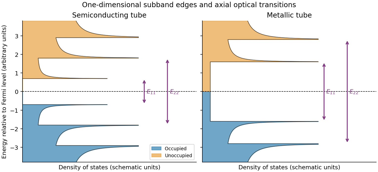
Rolling graphene into a single-walled carbon nanotube quantizes the circumferential wave vector, leaving a set of one-dimensional longitudinal subbands. At each subband edge the group velocity tends to zero, producing a Van Hove singularity in the density of states. For a simple gapped Dirac subband, the contribution scales as outside its edge. At low temperature the valence states below the Fermi level are occupied and the conduction states above it are empty. A semiconducting tube has a gap; an ideal metallic tube has gapless channels as well as higher-subband singularities.
For light polarized along the tube, the strongest allowed interband transitions connect corresponding subbands while approximately conserving axial wave vector and circumferential angular momentum. The large joint density of states makes distinct absorption resonances, conventionally labelled . Strong electron–hole interactions produce bound excitons, so the observed optical resonances differ from the noninteracting band separations. Defects, doping, bundling and dielectric screening change peak energies and oscillator strengths. The original schematic below depicts the subband-edge structure, not measured spectra.
Taking room temperature as , the thermal voltage is . For the stated ideal diode, , soThe term is negligible here. A different precise interpretation of room temperature changes the result noticeably because of the exponential; the calculation above states its temperature explicitly.
For a lower-bandgap material, the intrinsic carrier concentration generally rises, increasing the reverse saturation current density, approximately through with when other parameters are held comparable. Thus the forward electric current at the same voltage would normally increase. If were artificially held fixed at the supplied numerical value, however, the ideal-diode equation would give the same electric current: the band gap dependence enters through the material parameters rather than as a separate term in that equation.
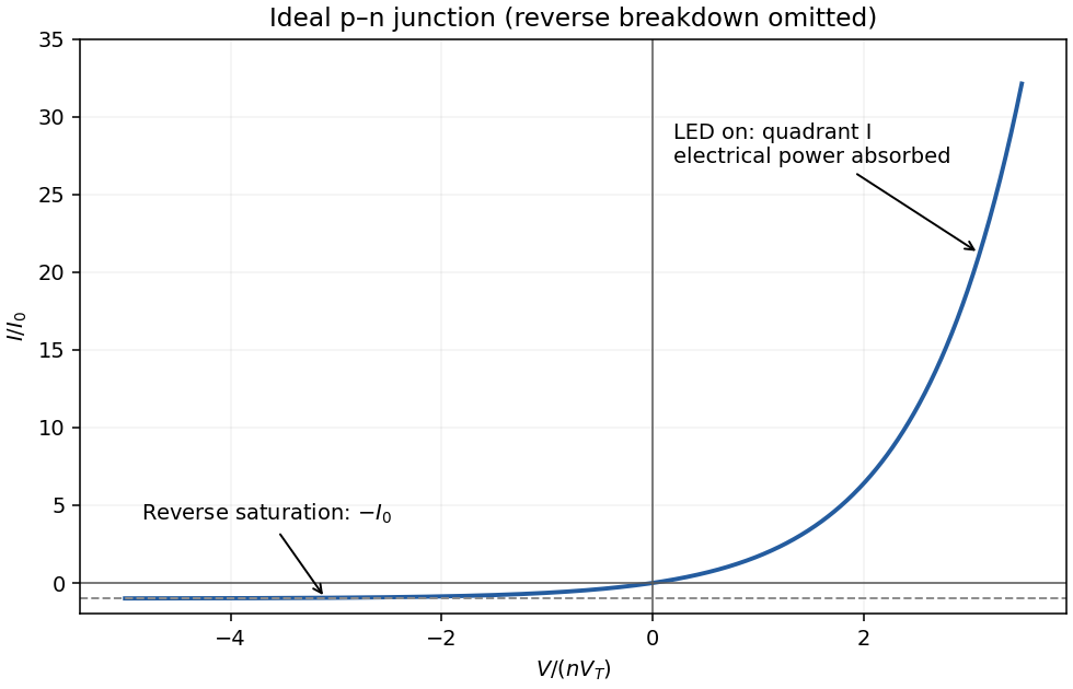
forward bias opposes the built-in electric field and lowers the junction barrier from approximately to . In the abrupt-junction depletion approximation,Thus the depletion region narrows and carriers cross the reduced barrier more readily. electron injection into the p side and hole injection into the n side increase strongly, allowing radiative recombination in an LED.
The injected minority-carrier concentrations, and therefore the ideal diffusion electric current, vary approximately as . This produces the steep forward branch of the electric current–voltage curve. One should not extrapolate the depletion-width formula to claim that the junction must lose its entire depletion region before conducting; appreciable electric current flows while a barrier remains, and high injection and series resistance eventually invalidate the simple formulas.
With conventional electric current defined into the positive terminal, an ideal junction hasThe reverse-bias branch tends to before breakdown. In forward bias the electric current rises exponentially; a visibly sharp “turn-on” is a convenient operating description rather than a discontinuity in the equation. A powered LED emits in quadrant I, where , and the device absorbs electrical power . Strong reverse breakdown lies outside the ideal curve below.


Use a patterned resist or hard mask and anisotropic chlorine-based reactive-ion etching, for example an appropriate inductively coupled plasma process for GaAs/AlGaAs. Ion-assisted removal gives a well-defined mesa with less lateral undercut than an isotropic wet etch. Control etch time or endpoint to obtain the specified approximately depth.
There are unlisted articles, also show them or only show them.