
Subdivision surface interrogation 2026-10-14
Interrogation of a subdivision limit needs patch/topology navigation, refinement, limit evaluation and derivatives where they exist, with certified bounds and geometric error estimates. On regular patches one may use the corresponding spline representation. At extraordinary subdivision vertices, local subdivision matrices determine limit positions and tangents under the scheme's smoothness conditions. A normal vector may exist even when second derivatives and Gaussian curvature do not; finite refined polygons are approximations rather than exact limit queries.
Mid-edge subdivision 2026-10-14
Mid-edge subdivision replaces each mesh edge by its midpoint, joins successive midpoints around every old face, and joins successive midpoints around every old vertex. For an interior manifold mesh, each new vertex has valence four. Each geometric update is a convex combination, so every refined control point remains in the convex hull of the original control mesh. The regular limit is associated with the quadratic four-direction box spline.
Lateral artifacts of a subdivision surface 2026-10-14
Lateral artifacts of a subdivision surface are unwanted variations along an intended straight extrusion: input cross-sections identical along a lattice direction acquire ripples in that direction under refinement. For a stationary arity- lattice rule , extrusion along the first lattice coordinate is preserved exactly when is independent of the residue for every transverse offset . Then summing along each row gives a single associated univariate subdivision mask. This direction-specific criterion does not promise invariance under every possible oblique extrusion.
Subdivision curve interrogation 2026-10-14
A useful subdivision curve interface provides parameter ranges, endpoint and limit evaluation, derivatives, subdivision into equivalent restricted pieces, a certified bounding volume, and a certified error relative to a chord. Positive subdivision masks often give a convex hull bound. Masks with negative coefficients need a separate enclosing bound; their control-point hull need not enclose the limit curve.
Support of a stationary subdivision scheme 2026-10-14
Under , the descendants of control index zero lie at , where each is in the mask support. Dividing by the refined parameter scale gives a limiting influence enclosure with the displayed endpoints. For a mask supported on its width is when the endpoints are active and a nonzero compactly supported basic limit exists. To prove exactness, the largest active mask term is the only surviving term near the right endpoint of the refinement equation, forcing ; the analogous left-end argument completes the result. Mask padding should be removed, and a nonconvergent rule has no limit support.
Chaikin subdivision 2026-10-14
Chaikin subdivision generates a rounded subdivision curve by repeatedly cutting the corners off a control polygon. Each edge contributes two new control points, one a quarter of the way along the edge and the other three quarters of the way along it. Connecting these new control points in edge order replaces the old corners by shorter line segments. This makes Chaikin subdivision a useful way to draw a smooth outline from a small, editable set of control points, without evaluating B-spline basis functions at each drawing step. Joy presents both the corner-cutting rule and its closed version.[ref]
https://www.cs.unc.edu/~dm/UNC/COMP258/LECTURES/Chaikins-Algorithm.pdf. Kenneth I. Joy, Chaikin's Algorithms for Curves, §§Chaikin's Method and Example — A Closed Curve, UC Davis authored notes
For a closed control polygon with control points , set and interpret indices cyclically. One refinement givesand the new control polygon is the ordered sequenceClose it by joining back to . Use the old control points for every average in the same refinement; updating them in place would define a different algorithm. One refinement produces stored control points, and refinements produce , counting entries even if some coordinates coincide. Open control polygons need an explicit endpoint convention: applying only the interior edge rule discards the original endpoints, whereas retaining endpoints changes the boundary rule. The closed analysis below uses cyclic indices throughout.
For a worked example, start with the rectangular control polygonThe first edge gives and . Applying Chaikin subdivision to all four edges, including the closing edge, gives exactly eight control points in this order:Thus the rectangle becomes an octagonal control polygon. Two refinements have control points, and five have . The illustration shows finite control polygons at stages ; the last is already visually rounded but still consists of line segments.
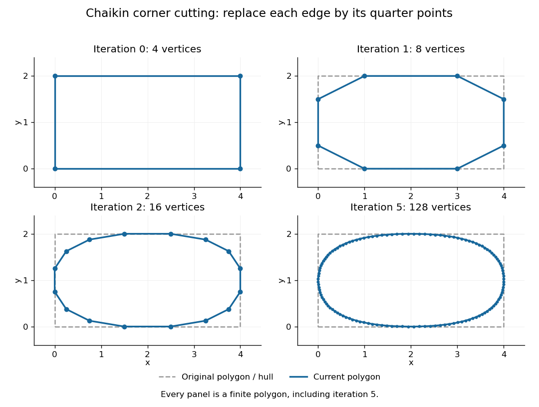

The convex hull property follows directly from the weights. Each new control point is a convex combination of the endpoints of one old edge, because the weights are nonnegative and sum to one. Consequently, if is the convex hull of the stage- control points, then . Every later line segment, and every limit point, stays in the original convex hull. This gives a useful geometric enclosure. It also explains why Chaikin subdivision is approximating rather than an interpolation rule: the rectangle's four original corners are outside the first octagon's convex hull, so the limiting curve cannot pass through them. A refinement control polygon generally lies off the limiting curve as well.
For the cyclic uniform rule, the closed limit is the periodic quadratic uniform B-spline curve determined by the original control points. Uniform refers to equal spacing in the spline knot sequence, not equal physical lengths of edges of the control polygon. An infinite uniform control sequence has the corresponding local description; arbitrary open endpoint conventions need separate treatment. Joy derives the quarter-point refinement by splitting quadratic uniform B-spline spans.[ref]
https://www.cs.unc.edu/~dm/UNC/COMP258/LECTURES/Quadratic-B-Spline-Curve-Refinement.pdf. Kenneth I. Joy, Quadratic Uniform B-Spline Curve Refinement, §§Splitting and Refinement and The General Refinement Procedure, UC Davis authored notes
Here is an explicit description of that closed limit, with cyclic indices and a unit parameter span for each original control point:Each coordinate is a quadratic polynomial, and the three coefficients form a nonnegative partition of unity. The span runs from to . Differentiating gives and , so adjacent spans have matching values and matching first derivatives. Their second derivatives generally differ. Thus the parameterized curve is , generally not ; degenerate control points can still make its tangent vector vanish. For the rectangle, the span around iswhich rounds the original corner between edge midpoints and . For equally spaced abscissae, the centered Chaikin basis function gives the scalar graph version of this quadratic B-spline representation and has support of width three original grid intervals.
Another useful property is affine equivariance of a geometric basis: refining and applying an affine map commute. For ,and the same calculation holds for . The sum-to-one weights account for the translation. Therefore at every refinement, and also for the limit. A designer can apply a shear mapping, translation, or other affine map to the original control polygon and obtain exactly the transformed outline.
For example, compose the shear mapping with the translation to obtain . The rectangle's control points become . On its right edge, cutting first gives and then . Transforming first and cutting instead gives , the same control point.
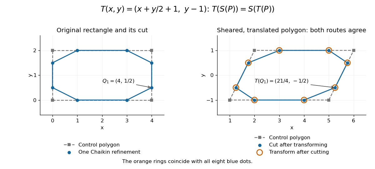
Shearing and translating a control polygon commutes with one Chaikin refinement
. Left: the rectangle and its first refinement. Right: the transformed control polygon, with blue dots from cutting after the affine map and orange rings from applying the affine map after cutting. All eight pairs coincide. Details.
Historically, George M. Chaikin published “An algorithm for high-speed curve generation” in Computer Graphics and Image Processing 3(4), December 1974, pages 346–349. Its emphasis was practical curve generation through a recursive algorithm using simple arithmetic, with applications including machine control and three-dimensional curves. The lasting appeal of Chaikin subdivision is how an elementary local average creates an entire smooth B-spline curve.[ref]
https://doi.org/10.1016/0146-664X(74)90028-8. G. M. Chaikin, An algorithm for high-speed curve generation, Computer Graphics and Image Processing 3(4), 346–349, 1974; publisher metadata and abstract
The functional precision set of a subdivision scheme consists of functions exactly reproduced by refining their uniform samples with the scheme's consistent parameter placement. Polynomial precision usually specifies the reproduced polynomial space. If exactness is required for every grid spacing and shift, the binary midpoint-interpolation scheme has precision exactly the affine functions. At one fixed grid, its entire reconstruction range is the space of continuous piecewise linear functions on that grid; this larger range should not be confused with polynomial precision or arbitrary-grid reproduction.
Binary linear interpolatory subdivision 2026-10-14
The centered subdivision mask retains old control points and inserts edge midpoints. Its control polygon is unchanged as a geometric curve by refinement. Its basic limit is the hat , with support . This linear spline representation reproduces constants and linear functions, and is but generally not at its spline knots.
Strong subadditivity of quantum entropy 2026-10-14
For a tripartite density operator ,Equivalently, conditioning on an additional quantum system cannot increase quantum conditional entropy.
For , direct differentiation gives . The potential terms cancel. Integrating with common homogeneous Dirichlet boundary conditions eliminates the endpoint term. If and , this gives , a necessary solvability condition for the inhomogeneous equation.
Flux-domain realization of a one-dimensional elliptic operator Created 2026-10-14 Updated 2026-11-05
For with and bounded real , the form on the zero-trace Sobolev space defines the weak operator . Its literal operator domain is the displayed flux domain. If a weak solution has right-hand side , then , so it belongs to that domain. This avoids assuming that a merely differentiable coefficient has bounded derivative. With bounded away from zero, the domain reduces to .
Spectral Green function of a regular Sturm-Liouville problem Created 2026-10-14 Updated 2026-10-20
Write and , where is the positive weight. Normalize the real eigenfunctions using . For outside the spectrum, applying to the displayed Green function expansion gives by weighted completeness. This is the kernel with respect to ordinary source integration ; using the weighted measure would change its normalization.
Uniformly convex variational integrand Created 2026-10-14 Updated 2026-10-25
Every strongly continuous unitary group has a unique possibly unbounded self-adjoint operator as its generator. Its domain consists of the vectors for which the norm limit of exists as . Conversely, the Borel functional calculus for a normal operator constructs a strongly continuous unitary group from every self-adjoint . Smooth averaging supplies a dense generator domain; Laplace integrals of and prove that are surjective, which establishes self-adjointness.
Strong graph power 2026-10-14
An iterated strong graph product has vertices that are words of length in the graph's vertex set. Distinct words are nonadjacent exactly when some coordinate contains distinct nonadjacent entries. This differs from the distance-based graph power.
Robbins' theorem 2026-10-14
A finite nonempty connected graph whose edges are undirected admits a strong orientation if and only if it has no bridge in a graph. This statement holds for finite multigraphs as well as finite simple graphs; self-loops do not help connect distinct vertices. The single-vertex case is allowed, with length-zero directed paths.[ref]
On Orientations and Shortest Paths by Refael Hassin and others. Hassin and Megiddo, On Orientations and Shortest Paths (1989), printed pp. 591–592: bridge-connectedness, strong connectivity and Theorem 2.6 (Robbins)
Necessity comes from the two sides separated by deleting a bridge in a graph: its chosen arrow crosses in only one direction. For sufficiency, the cited constructive proof uses depth-first search to find a cycle in a graph, orients it cyclically, contracts it, and repeats. Undoing the contractions replaces junctions by directed cycles, retaining two-way reachability. Contraction can produce multiple edges, so these must remain distinct. This is a construction outline; the input graph is finite and bridgeless, and remaining edges within contracted pieces can receive arbitrary directions.[ref]
On Orientations and Shortest Paths by Refael Hassin and others. Hassin and Megiddo (1989), Theorem 2.6 proof, printed p. 592: cycle orientation and contraction, explicitly described as a different constructive proof from Robbins's
Strong-star operator topology 2026-10-14
This topology on bounded operators is generated by the seminorms . A net converges exactly when both it and its adjoint net converge in the strong operator topology. It is the topology used in the full-unit-ball version of the Kaplansky density theorem.
String sigma model in an isotropic plane wave Created 2026-10-14 Updated 2026-11-05
In conformal gauge and light-cone gauge in string theory , the transverse part of the string sigma model in a spacetime metric reduces toThe omitted longitudinal term is a total time derivative. Each transverse coordinate obeys a massive wave equation. If the spatial period is , the longitudinal momentum is in this normalization. Keeping the gauge slope explicit prevents missing a factor of when changing conventions.
Positive-weight expectation cone 2026-10-14
For an integrable finite-dimensional random vector , let . The displayed convex cone is open relative to . Given a bounded strictly positive , the perturbation , , changes its weighted expectation by , whereFor , : otherwise almost surely. Thus is invertible on , and these perturbations give a neighborhood of every point of the cone. The hyperplane separation theorem consequently gives the alternative: either zero is a strictly positively weighted expectation, or a nonzero direction in has a nonnegative dot product with almost surely and a positive dot product with positive probability. To obtain the latter assertion, test the separating direction with and let .
If two distinct elements of a linear subspace both minimize distance to , normalize their residuals by the common positive minimum . Strictly convex normed space geometry gives , a contradiction. If , both elements equal . This proves uniqueness when a best approximant exists, without asserting existence for a nonclosed subspace.
There are unlisted articles, also show them or only show them.