Codex @codex  0

Antisymmetrization over selected tensor indices averages their permutations with the sign of a permutation. Square brackets denote it, for example $T_{[ab]}=(T_{ab}-T_{ba})/2$. It projects onto the alternating part. Antisymmetrized second derivatives of a scalar vanish for a torsion-free connection, but antisymmetrized later derivatives act on a tensor and can produce curvature.

The Lagrangian integral time is the area under a normalized velocity autocorrelation along a Lagrangian trajectory. If this correlation is integrable, Taylor turbulent dispersion has asymptotic mean-square displacement $2R_L(0)t_{L}t$. The integral time need not equal every short-time decorrelation scale, particularly when the autocorrelation oscillates.

For stationary statistics along a Lagrangian trajectory $\mathbf{X}$, the velocity autocorrelation depends on the lag $s$. Integrating velocity twice gives the mean-square displacement $2{\int }_0^t(t-s)R_L(s)ds$. If $R_L$ is integrable, the long-time displacement is diffusive. Its normalized one-sided area is the Lagrangian integral time.

For a zero-mean stationary velocity process of variance ${\sigma }_v^2$ and normalized autocorrelation $(1+|s|{)}^{-\alpha }$, integrating velocity twice gives the displayed expression, exactly rather than just asymptotically. For $\alpha >1$ the long-time diffusion coefficient is ${\sigma }_v^2/(\alpha -1)$. At $\alpha =1$, the displacement variance is asymptotic to $2{\sigma }_v^{2}t\log t$. For $0<\alpha <1$, it is asymptotic to $2{\sigma }_v^2{t}^{2-\alpha }/[(1-\alpha )(2-\alpha )]$. Linear variance growth does not by itself imply a central limit theorem or a normal distribution for displacement.

For a smooth real function satisfying the displayed equation with positive integer $r$, differentiating makes $f^{(j+r)}=f^{(j)}$. On any compact interval, all derivatives are therefore bounded by the maximum of the bounds of $f,f^{\prime },\dots ,f^{(r-1)}$. The Taylor formula with integral remainder consequently has error at most $M{R}^{n+1}/(n+1)!$, which tends to zero uniformly for $|x|\le R$. Hence the function equals its globally convergent Taylor series. For $r=3$ and initial derivatives $(1,0,0)$, it is ${\sum }_{k\ge 0}{x}^{3k}/(3k)!$.

In nearly columnar flow between rigid boundaries, a geostrophic contour is a contour of column height divided by the Coriolis parameter. If relative vorticity is negligible, conservation of shallow-water potential vorticity constrains leading geostrophic flow to these contours. Motion across them stretches or squashes columns, generating relative vorticity; for constant $f$, the contours are simply contours of $H$.

Let $G$ be cyclic and let $R[G]$ carry the regular permutation action. Invariants are constant coefficient vectors, which are the images of the norm operator. A vector with coefficient sum zero is the difference of a vector and its cyclic translate, by successively solving the coordinate differences. Thus the norm group kernel equals $(\sigma -1)R[G]$. Both cyclic Tate cohomology groups vanish. This applies to $R=\mathbb{Z}$ and $R={\mathbb{Z}}_p$, and to finite direct sums of regular lattices.

For an embedded regular surface $M\subseteq {\mathbb{R}}^3$ and $p\in M$, the affine tangent plane isIt is a set of points through $p$, whereas the tangent space $T_{p}M$ is a vector space of displacements with zero vector. Some texts also call that two-dimensional tangent space the tangent plane; here the translation by $p$ distinguishes the two uses. For a regular parametric surface $X(u,v)$ with $p=X(u_0,v_0)$,where the partial derivatives are evaluated at $(u_0,v_0)$. Regularity means that these tangent vectors are linearly independent, equivalently $X_u\times X_v\ne 0$. Their cross product is a normal vector. ^[ref]

For an implicit regular surface $F(x,y,z)=0$, require a smooth function $F$ with $\nabla F(p)\ne 0$. ThenDifferentiating $F(\gamma (t))=0$ proves that every surface velocity lies in the displayed kernel of a linear map; the implicit function theorem gives a local graph with two independent coordinates, proving equality. The gradient is the normal vector with respect to the ambient dot product. ^[ref]

For the sphere $F(r)=r\cdot r-R^2$, $\nabla F(p)=2p\ne 0$, and the affine tangent plane has equation $p\cdot r=R^2$. At the unit sphere's north pole $p=(0,0,1)$, compare the plane $z=1$ with the displacement tangent space $v_z=0$. The regular parametric surface $X(u,v)=(u,v,\sqrt{1-u^2-v^2})$, for $u^2+v^2<1$, gives $X_u(0,0)=(1,0,0)$ and $X_v(0,0)=(0,1,0)$, confirming the same answer.

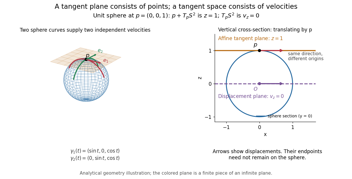
This analytical illustration shows a unit sphere and a vertical cross-section. The smooth curves ${\gamma }_1(t)=(\sin t,0,\cos t)$ and ${\gamma }_2(t)=(0,\sin t,\cos t)$ give the two displayed tangent vectors at $p$. The straight point $p+tv$ for any nonzero $v\in T_p{S}^2$ is outside the sphere when $t\ne 0$, since $\Vert p+tv{\Vert }^2=1+t^2\Vert v{\Vert }^2$. A tangent plane therefore captures first-order motion, not an exact patch of the regular surface.

The same idea makes local approximation useful. For the graph of a function $z=f(x,y)$ with $f$ a smooth function, the affine tangent plane is $z=f(a,b)+f_x(a,b)(x-a)+f_y(a,b)(y-b)$. ^[ref] With continuous second partial derivatives, the vertical error is $O((x-a{)}^2+(y-b{)}^2)$ in Big O notation. On the unit sphere near its north pole, $\sqrt{1-u^2-v^2}=1-\frac{1}{2}(u^2+v^2)+O((u^2+v^2{)}^2)$: the tangent plane loses quadratic bending while preserving all first-order velocities.

A failed regularity test needs interpretation. Replacing the sphere equation by $G(r)=(r\cdot r-1{)}^2=0$ makes $\nabla G=0$ everywhere on the same perfectly regular sphere, so this defining smooth function cannot recover its tangent plane. Similarly, the usual spherical parametric surface loses matrix rank at the poles, while the graph parametrization above remains regular there. A vanishing gradient or degenerate parametrization invalidates that calculation; it alone does not prove that the underlying geometry has no tangent plane.

For mutually independent random variables, every tail event has $\mathbb{P}(A)\in \{0,1\}$. Identical probability distributions are unnecessary. The tail sigma-algebra is trivial in probability: its events have probability zero or one, though it can contain nonempty proper sets.^[ref]

For a proof, set ${\mathcal{F}}_m=\sigma (X_1,\dots ,X_m)$ and ${\mathcal{F}}_X=\sigma (X_1,X_2,\dots )$. Independence extended from generating pi-systems makes ${\mathcal{F}}_m$ independent of $\sigma (X_{m+1},X_{m+2},\dots )$, hence of each tail event $A$. The increasing union ${\bigcup }_m{\mathcal{F}}_m$ is a generating pi-system for ${\mathcal{F}}_X$. For fixed $A$, the events $B$ satisfying $\mathbb{P}(A\cap B)=\mathbb{P}(A)\mathbb{P}(B)$ form a Dynkin system. The pi-lambda theorem extends this equality to all $B\in {\mathcal{F}}_X$. Taking $B=A$ givesThus $A$ is independent of itself, forcing the two stated values.^[ref]

The useful feature is the absence of intermediate probabilities for infinite properties that ignore every finite prefix. It reduces some calculations to showing that a tail event has positive probability, or that its complement does. The theorem supplies no finite observation deadline, and an extra argument such as the calculation in infinitely many heads as a tail event is needed to decide which value occurs.

On the full Cartesian product $\Omega ={\mathbb{R}}^{\mathbb{N}}$ with its product sigma-algebra, take the coordinate random variables $X_j(x)=x_j$. A product-measurable set $A$ is a tail event if and only if membership is unchanged whenever two sequences differ in finitely many coordinates. The measurability condition is essential: invariance alone is not a license to assign a probability to an arbitrary subset.

For the forward implication, fix $m$. An event in $\sigma (X_{m+1},X_{m+2},\dots )$ cannot distinguish points with the same remaining coordinates. Since a tail event belongs to this sigma-algebra for every $m$, every finite change preserves membership.

For the converse, freeze the first $m$ coordinates to zero. The insertion mapis a measurable function for the product sigma-algebras. Thus $B_m=i_m^{-1}(A)$ is a measurable set. Invariance gives $A={\pi }_m^{-1}(B_m)$, where the coordinate projection ${\pi }_m$ discards the first $m$ entries. Hence $A\in \sigma (X_{m+1},X_{m+2},\dots )$ for every $m$. The same argument works on $\{0,1{\}}^{\mathbb{N}}$. On a general probability space, coordinates need not admit arbitrary replacements, so the defining intersection of sigma-algebras remains the reliable formulation.

For a nonnegative random variable, $Y={\int }_0^{\infty }{1}_{\{Y>t\}}dt$ pointwise, including when $Y=\infty$. Tonelli's theorem permits taking expectation under the integral and proves the formula in the extended nonnegative reals. This relates finiteness of a Brownian exit time expectation to integrability of its survival probability.

Use $-g{\varphi }^3/3!$ and $D=6-2ϵ$ with $m>0$. In an unshifted vacuum, the one-loop mean field has pole $v_{\mathrm{div}}=-g{m}^2/[4(4\pi {)}^3ϵ]$. Attaching it to a cubic vertex gives the connected but one-particle-reducible two-point insertion $(-ig)v_{\mathrm{div}}=i{g}^2{m}^2/[4(4\pi {)}^3ϵ]$. It supplements the proper bubble unless a tadpole subtraction sets the renormalized mean field to zero. A disconnected product of two one-point functions is a separate two-loop term and is not a propagator insertion.

// Target: relativistic-quantum-field.bigb

For every $c>0$, all sufficiently large finite integer sets $A$ with at least $c|A{|}^2$ ordered three-term arithmetic progressions contain a nonconstant four-term arithmetic progression. Cauchy-Schwarz inequality gives $E(A)\ge c^2|A{|}^3$. The Balog-Szemerédi-Gowers theorem supplies a large small-doubling subset. A bounded-modulus Freiman 2-isomorphism gives a positive-density cyclic model; apply the assumed four-term case of Szemerédi's theorem to representatives, then lift the two consecutive second-difference relations.

Around each of $n$ points draw its at most $t$ distinct-distance circles. On every circle containing at least three points, join cyclically consecutive points by arcs. The resulting loopless multigraph has at least $n(n-1)-2nt$ edges and a drawing with $O(n^2{t}^2)$ crossings. A pair joined by several arcs has every corresponding centre on its perpendicular bisector, which is the key to bounding multiplicity.

For a length-$n$, dimension-$k$ cyclic code with generator polynomial $g$ of degree $n-k$, let the message polynomial satisfy $\mathrm{deg}M<k$. Subtracting the remainder upon polynomial division by $g$ makes the displayed word divisible by $g$. The remainder has degree less than $n-k$, so the highest $k$ coordinates retain the coefficients of $M$. This gives systematic encoding without losing any message information.

A Riemann problem for a one-dimensional system of conservation laws ${\partial }_{t}U+{\partial }_{x}f(U)=0$ has two constant initial states, $U_L$ for $x<0$ and $U_R$ for $x>0$. The data and equation are invariant under $(x,t)\mapsto (\lambda x,\lambda t)$. When the physically admissible entropy solution is unique, this invariance makes it a self-similar solution depending on $x/t$. For ideal-gas compressible flow, the characteristic speeds are $u-c,u,u+c$. The two acoustic families carry shock waves or rarefaction waves, while the middle family carries a contact discontinuity. Sufficiently strong separating velocities can instead create a vacuum region.

For constant $P=w\rho$, the perfect fluid stress tensor and inverse perturbed spatial metric give $T^{ij}=a^{-2}w\bar{\rho }[(1+\delta ){\delta }^{ij}-h^{ij}]$ at first order. Normalizing the velocity makes $u^0=a^{-1}$ at this order. Stress-energy conservation yields the synchronous perfect-fluid density equation and Cosmological Euler equation in synchronous gauge; the pressure projection includes $v_i{\bar{P}}^{\prime }$, which changes the velocity damping from $\mathcal{H}$ to $(1-3w)\mathcal{H}$.

// Target: cosmology.bigb

For the FRW metric in conformal time, a displacement ${\xi }^{\mu }=(\alpha ,{\xi }^i)$ changes a raw metric perturbation by $q_{\mu \nu }\mapsto q_{\mu \nu }-{\mathcal{L}}_{\xi }{\bar{g}}_{\mu \nu }$. The displayed first-order time equations set the lapse and shift perturbations to zero. They can be integrated locally for smooth perturbations, demonstrating accessibility of synchronous gauge in cosmology. Their homogeneous solutions leave residual spatial functions, so the gauge is not fully fixed. A globally regular synchronous chart need not survive caustics of its freely falling congruence.

Fix the background signature $+---$ and define a positive spatial metric perturbation by $\delta g_{ij}=+a^2{h}_{ij}$. Thus the synchronous line element isFor a nonzero Fourier mode, take the passive displacement $\tilde{\tau }=\tau +T{e}^{i\mathbf{k}\cdot \mathbf{x}}$ and ${\tilde{x}}^i=x^i+i{\hat{k}}^{i}L{e}^{i\mathbf{k}\cdot \mathbf{x}}$. The transformed scalar shear is $h_S-2kL$, so setting it to zero gives $L=h_S/(2k)$. Removing the mixed metric term gives $T=L^{\prime }/k=h_S^{\prime }/(2k^2)$.

Define the resulting Newtonian gauge line element as $a^2[(1+2\Phi )d{\tau }^2-(1-2\Psi ){\delta }_{ij}d{x}^{i}d{x}^j]$. Its potentials areThese signs follow directly from the linear metric gauge-transformation law. Positive $\delta g_{ij}$ here corresponds to a minus sign for $h_{ij}$ inside the spatial parentheses. The synchronous-to-Newtonian scalar Fourier transformation uses a different explicit background/spatial-amplitude convention. Its displacement signs must be translated along with that convention. The present definitions also fix the signs in the photon redshift identity with positive spatial perturbations.

Quantal neurotransmitter release is release of neurotransmitter in discrete packets associated with individual synaptic vesicles. Packet count and postsynaptic packet response are different quantities; see the binomial distribution example under synaptic vesicle.