
Orientation of a smooth manifold 2026-10-14
An orientation of a smooth manifold is a continuous choice of orientation of a vector space in every tangent space, equivalently an orientation of a vector bundle on its tangent bundle. It can be specified by an atlas with positive Jacobian determinants on all overlaps or by a nowhere-vanishing top-degree differential form. On a connected orientable manifold there are two choices, interchanged by reversing every tangent-space orientation.
// Target: differential-geometry.bigb
Left Ore fraction construction 2026-10-14
For a multiplicative set of regular elements satisfying the left Ore condition, represent a fraction by . Pairs and agree when there are with and . Addition uses this common denominator. For multiplication choose with , then . The Ore condition gives common multiples for successive operations; regularity supplies cancellation. In a domain with all nonzero elements, every nonzero fraction has inverse .
// Destination: associative-algebra.bigb
If two nonzero principal right ideals in a right Noetherian domain had zero intersection, the sums would be strictly increasing. Directness follows by splitting the lowest term into and the other terms into , then cancelling and repeating. This contradicts the ascending chain condition. A nonzero common element gives the right Ore condition. The left version follows from the opposite ring. Consequently a noncommutative domain Noetherian on both sides has a single division ring of fractions with both left and right fraction presentations.
Classical left ring of quotients Created 2026-10-14 Updated 2026-11-05
This is the localization of a ring at all its regular elements of a ring, with left fractions. It exists precisely when those denominators satisfy the left Ore condition. If embeds in a ring , all regular elements become units in , and every element of is such a fraction, the Ore condition follows by writing , which gives .
In the ordinary topology on infinite subsets, the family of cofinite sets is a countable set, a dense and a meagre set. Countability follows by indexing its members by their finite complements. Each singleton is closed with empty interior, while every basic cylinder with finite initial segment contains . Consequently is not a nowhere dense set. This example uses the ordinary cylinder topology, rather than the Ramsey cone topology.
Ordinal division algorithm 2026-10-14
For ordinals and , there are unique ordinals with the displayed relation. The function is strictly increasing, continuous at limit ordinals and unbounded. Its first value above occurs at a successor, giving the largest with . The ordered tail of after that initial segment gives , and maximality gives .
Fast-growing hierarchy 2026-10-14
A fast-growing hierarchy indexes number-theoretic functions by an effective system of ordinal notations. Successor stages iterate the preceding function, while limit stages diagonalize along a chosen fundamental sequence of a limit ordinal. These choices are part of the definition. With the standard Cantor normal form sequences below epsilon zero, each fixed for is provably total in Peano arithmetic, but the uniform endpoint is not. Every function provably total in Peano arithmetic is eventually bounded by some lower level. These classification results are proved in epub.ub.uni-muenchen.de/3843/1/3843.pdf .
Fundamental sequence of a limit ordinal Created 2026-10-14 Updated 2026-10-20
For a countable limit ordinal, a fundamental sequence is an increasing cofinal sequence of smaller ordinals. Effective choices allow a fast-growing hierarchy to turn limit recursion into recursion at a finite input. Below epsilon zero, write the final term as . For successor , take ; for nonzero limit , take . Earlier terms in the Cantor normal form remain fixed.
Covariance of Grassmann bilinears Created 2026-10-14 Updated 2026-11-05
For , ordered Grassmann Gaussian contractions give and . The disconnected contribution has two fermion loops; the connected contribution has one, giving its minus sign. This covariance is an algebraic normalized Berezin integral, rather than a positivity statement about a probability measure.
First ascent in independent continuous observations Created 2026-10-14 Updated 2026-11-05
For independent and identically distributed random variables with a continuous probability distribution, let be the index of the first increase. The event requires the first observations to be decreasing; symmetry among their possible strict orders gives probability for . Subtracting successive tails gives the displayed mass function for . The tails tend to zero, so is finite almost surely. The tail-sum formula for expectation gives , independently of the continuous sampling law.
Pseudo-first-order reaction 2026-10-14
In a second-order reaction with rate law , a large excess of B can keep during the observation window. ThenThis is a pseudo-first-order reaction: the approximate first-order reaction describes that window, while changing the excess B concentration changes . Its units are , distinct from the second-order reaction rate constant . For one-to-one stoichiometry, the maximum fractional depletion of B is ; an original initial excess bounds its change by . A twofold excess permits depletion and does not provide the same control.[ref]
Glossary of Terms Used in Physical Organic Chemistry (IUPAC Recommendations 1994): N and O entries by International Union of Pure and Applied Chemistry. Glossary of Terms Used in Physical Organic Chemistry, IUPAC Recommendations 1994, entry “order of reaction”: constant B, observed coefficient and pseudo-first-order coefficient
Second-order reaction 2026-10-14
A second-order reaction has overall order of reaction two: a rate law may depend on , or on with partial orders of reaction one and one. Doubling all relevant reactant concentrations multiplies the reaction rate by four at fixed conditions. This experimentally determined dependence does not establish molecularity or a unique reaction mechanism. For an elementary reaction obeying the law of mass action, molecularity and overall order of reaction agree; a net chemical equation alone cannot establish that the conversion is elementary.[ref]
Glossary of Terms Used in Physical Organic Chemistry (IUPAC Recommendations 1994): N and O entries by International Union of Pure and Applied Chemistry. Glossary of Terms Used in Physical Organic Chemistry, IUPAC Recommendations 1994, entry “order of reaction”, final paragraphs: elementary versus stepwise reactions
For the single-concentration model, explicitly choose the disappearance rate conventionHere is the coefficient for loss of A, held fixed at the specified temperature and other conditions. Its subscript labels the chosen observed disappearance rate; it does not imply a pseudo-first-order reaction. Assume a uniformly mixed closed system, fixed volume, and no appreciable reverse or competing chemical reactions. The integrated rate law isThe reciprocal-concentration plot is a straight line with slope and intercept . A brief derivation uses the chain rule: , then applies the initial condition. This is a hyperbolic decay, rather than the exponential decay of a first-order reaction.[ref]
Chemistry 2e. §12.4, “Second-Order Reactions”, integrated equation and straight-line form; Table 12.2
As an original prescribed example, choose and . At , the reciprocal-concentration calculation is , giving . The initial disappearance rate is ; after it is . Halving the concentration quarters the disappearance rate.
Dimensional analysis checks every formula: has units , has units , and is a dimensionless quantity. Changing concentration units changes the numerical rate constant: the same example is , , giving .
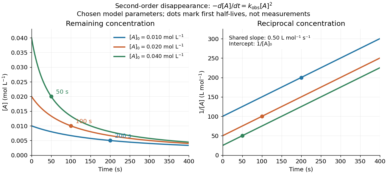
Second-order reaction concentration decay and reciprocal-concentration lines for three prescribed starting concentrations
. Original model curves, not measured data. All use the disappearance rate coefficient . The reciprocal lines share a slope while their intercepts differ; marked points give each run's first half-life. Details.
For an elementary reaction , instead define the stoichiometrically normalized reaction rate . Two A entities disappear per P formed, soConsequently the reciprocal-concentration slope is , not . In the prescribed example, the normalized rate constant would be ; initially while the disappearance rate is twice that. With , stoichiometry gives . Both rate constants have the same dimensions, so a units check alone cannot catch their factor-of-two difference. The symbol denotes the same normalization as in reaction rate.
The half-life, meaning the time to reach half a specified starting concentration, follows by setting :For in , this becomes . Its units are seconds because has units . Doubling the starting concentration halves the first half-life; a quoted half-life needs its starting concentration. This differs from a first-order reaction, whose half-life is independent of starting concentration.[ref]
Within the prescribed run, reaches , , and at , , and . The successive halving intervals are , , and : each begins at a smaller concentration. More generally, reaching fraction of the initial concentration, with , requires , so consumption takes nine initial half-lives, rather than a fixed sequence of equal waiting times.
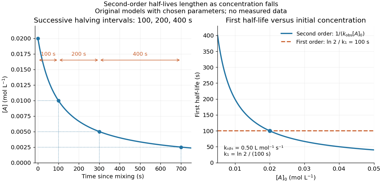
Lengthening second-order reaction halving intervals and the dependence of the first half-life on initial concentration
. Original model predictions, not measurements. Left: the prescribed run. Right: at fixed , compared with a first-order reaction chosen to have . That comparison uses , with different units from . Details.
A straight reciprocal-concentration plot tests this particular single-concentration rate equation. It does not uniquely identify a reaction mechanism, nor does curvature rule out every second-order reaction: two independently changing reactant concentrations require their own integrated rate law. At low concentration, a small measurement error becomes approximately in the reciprocal, magnifying late-time errors. Use the line as a diagnostic; a nonlinear regression of the original concentrations can retain their measurement scale and explicit error model.
Zero-order reaction 2026-10-14
A zero-order reaction has a reaction rate independent of the relevant reactant concentration over the range where its rate law applies. For , is valid only before depletion at . The constant-consumption model must stop or change there.
First-order reaction 2026-10-14
A first-order reaction has a reaction rate proportional to one reactant concentration in the simple single-species case. For an irreversible in a closed system at fixed volume, take , , and constant rate constant . Its rate equation and solution areA short check is enough: differentiating gives , and the two concentrations sum to , as required by the one-to-one stoichiometry. Thus the same exponential decay describes both remaining reactant and decreasing reaction rate. Fixed means a fixed fractional loss per unit time, not a fixed absolute consumption rate.
Choose illustrative values and , with measured in seconds. Then , , and . The half-life isAt each successive half-life, half the remaining reactant is consumed; is independent of for this first-order reaction. At , the calculated values are , , and . These are model predictions for chosen parameters, rather than experimental measurements.
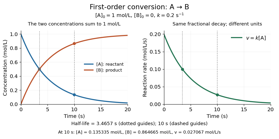
Illustrative first-order reaction: reactant loss, reaction product formation, and declining reaction rate for
. Details. 
The left panel tracks the two concentrations; the right tracks their instantaneous conversion reaction rate. Their different vertical units matter: , so the numerical curves need not have the same height. This gives a practical way to translate a measured concentration into a forecast of both conversion and waiting time.
Zero sets in the unit disc 2026-10-14
A nonzero holomorphic function on the unit disc can have exactly a prescribed sequence of zeros, counted with multiplicity, if and only if that sequence is locally finite in the disc. Necessity is the identity theorem for holomorphic functions. For sufficiency, remove a finite number of zeros at zero and enumerate the others as , so . Use the Weierstrass elementary factors . On every compact subdisc, eventually and . Hence converges locally uniformly and has exactly the prescribed zeros. Finite sequences simply give finite products.
True longitude 2026-10-14
True longitude is the conventional orbital angle formed from the longitude of ascending node, argument of periapsis and true anomaly. For a coplanar Kepler orbit it is the actual polar longitude of the position vector. For an inclined orbital plane the sum of angles is generally not the projected azimuth. The mean longitude uses mean anomaly in place of , so . For small orbital eccentricity, Kepler's equation gives , while the eccentric-to-true anomaly relation gives ; hence . This periodic difference matters when separating a slow resonant argument from a rapidly varying geometric angle.
Argument of periapsis Created 2026-10-14 Updated 2026-10-18
The argument of periapsis is the angle in the orbital plane from the ascending node to periapsis, measured in the direction of motion. It differs from the longitude of periapsis . For an inclined orbit this sum is a conventional longitude, not generally the azimuth of the projected periapsis. The argument is undefined for a circular orbit and the node-based description is singular when the orbit and reference plane coincide.
Equality-pattern orbits of ordered pairs Created 2026-10-14 Updated 2026-11-05
The diagonal group action of the symmetric group on ordered pairs has two orbits of a group action when : equal pairs, of size , and distinct pairs, of size . Equality is preserved by a bijection, and a prescribed bijection on one or two distinct letters extends to a permutation of all letters. At only the equal-pair orbit remains.
Call delta equation for a driftless local volatility diffusion Created 2026-10-14 Updated 2026-11-05
In the cash-numéraire market , let a smooth call value solve . Its delta hedge is . Differentiating the pricing equation giveswith this terminal condition interpreted away from . If the terminal law has no atom at , its assigned value at that point does not affect expectation pricing; a degenerate or absorbed diffusion can instead require a separate strike-boundary analysis. By Itô formula, , while . Thus holding shares and cash replicates the terminal call. The drift in the option delta equation comes from differentiating the spatially varying diffusion coefficient, not from a drift in the original stock.
For an equiprobable source, an optimal binary prefix tree has leaf depths differing by at most one. If one leaf has depth and a deepest sibling pair has depth , split the shallow leaf into two children and collapse the deep pair into its parent. The number of leaves is unchanged and their total depth decreases by , contradicting optimality.
// Target: probability-and-statistics.bigb
There are unlisted articles, also show them or only show them.