
Node (physics) 2026-10-14
A node of an ideal standing wave is a position whose oscillation amplitude is zero: its displacement stays zero for all time. For a nontrivial normal mode , this means . A momentary zero caused by does not make every position a node. In more dimensions the zeros of a mode shape can form curves or surfaces.
For the th normal mode of a uniform fixed-end wave equation on a string, the nodes of a standing wave areThere are nodes of a standing wave including the two endpoints, and interior ones. For and , they lie at , , , and . Each remains stationary through every snapshot in the normal mode diagram; an antinode instead marks a maximum oscillation amplitude. [ref]
Normal-mode energy exchange 2026-10-14
For the undamped first normal mode of a fixed string, start at maximum displacement with . In the small-slope wave equation on a string, its kinetic energy and excess potential energy areThe potential energy comes from the extra length under tension: . It depends on slope, so a node of a standing wave need not have zero local potential energy density. These are physical energies, with the mass and tension factors restored to the normalized wave energy. [ref]
https://farside.ph.utexas.edu/teaching/315/Waveshtml/node43.html. Richard Fitzpatrick, Oscillations and Waves, Energy Conservation, equations 6.24-6.29
Integrating and over the string gives in both cases. Using yieldsFor the model , , , and , the angular frequency is , the frequency is , and . The maximum slope is small. At all the energy is potential energy; at the string is straight and all the energy is kinetic energy. At the displacement is reversed and all the energy is again potential energy. The energy curves repeat twice during one displacement cycle, while conservation of energy keeps their sum constant.
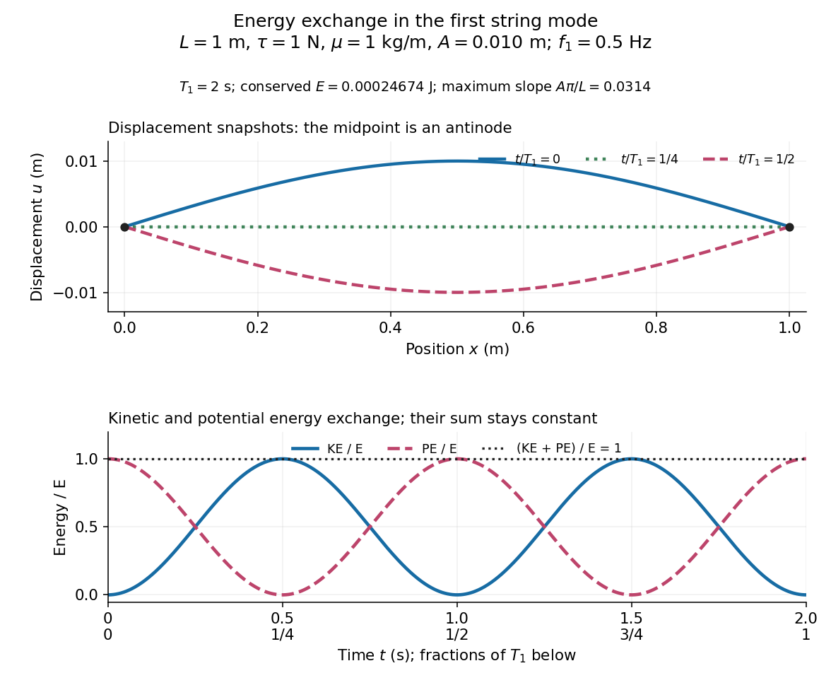
First-mode displacement in metres and kinetic and potential energies divided by the conserved total energy
. Details. Countability of elastic eigenfrequencies 2026-10-14
Distinct squared traction-free eigenfrequencies in a bounded lossless elastic body have eigenfunctions orthogonal in , by the Betti identity for elastodynamic fields. Normalize one field from each eigenspace. This is an orthonormal set in a separable Hilbert space, so it is countable: disjoint balls of radius less than around its unit vectors must contain distinct points of a countable dense set. Positive and negative frequency partners add at most a factor of two. This argument proves countability without requiring a separate compact-resolvent proof.
Mode shape Created 2026-10-14 Updated 2026-10-18
The mode shape is the fixed spatial eigenfunction multiplying the temporal factor of a normal mode. It is determined by the governing differential equation and boundary conditions, and may be normalized by a chosen amplitude or energy convention.
For the same normal distribution model, a two-sided test compares the null hypothesis with the alternative hypothesis . Under the null hypothesis, the standardized test statistic has standard normal distribution. Write for the standard normal distribution function. With , , and , the observed test statistic is . Its p-value isThus the p-value is a tail probability computed under the null hypothesis, including departures in both directions. It is not , the posterior probability of the null hypothesis, nor the probability that the observations arose "by chance". The normal distribution test statistic and its calibration appear in NIST's teaching reference for testing a process mean; the tail interpretation is stated in Penn State's hypothesis-testing notes.
Choose the significance level before observing the sample. The rejection region is , whose probability under is exactly 0.05. Here , so reject . This agrees with zero lying outside . More generally, a proposed belongs to the unrounded 95% confidence interval precisely when its two-sided test does not reject under this strict cutoff. The equality boundary has probability zero in this continuous statistical model.
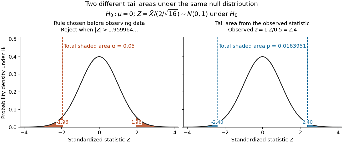


The significance level and statistical power describe different repeated-experiment probabilities. At a specified alternative , put and . ThenThe first is the Type I error probability; the second is the Type II error probability at that alternative. For a planning alternative , keeping , and gives , and statistical power . At , and statistical power rises to . These are model calculations for specified alternatives, not posterior probabilities inferred from a nonsignificant result. They explain why failure to reject cannot establish equality and why choosing sample size before an experiment is useful.
Historically, Ronald Fisher's 1925 book discusses the normal cutoff and tail probability 0.05 as a convenient convention on page 47, rather than a mathematically compulsory threshold: [ref]
https://books.google.com/books/about/Statistical_Methods_for_Research_Workers.html?id=I0NBAAAAIAAJ. Fisher, Statistical Methods for Research Workers, first edition
. Normal matrices have equal adjoint norms 2026-10-14
For a normal matrix, . Consequently . In particular, and its Hermitian conjugate have the same kernel of a linear map.
Pure error 2026-10-14
With repeated responses at an identical predictor configuration, pure error is their within-configuration variability. Its residual sum of squares can estimate measurement variance independently of a candidate regression mean function. Without replication, a fitted residual can combine pure error and lack of fit.
Lack of fit 2026-10-14
Lack of fit is a mismatch between a regression model's mean function and the true mean relationship. Replicated predictor configurations can separate its sum of squares from pure error. A residual-versus-fitted plot can suggest curvature or changing variance even without a formal replication-based test.
For a full-column-rank design and with , the maximum-likelihood estimators are and . Orthogonal Gaussian projections give their displayed distributions and independence. The variance maximum-likelihood estimator has expectation ; the unbiased residual variance divides by instead.
Analysis of covariance 2026-10-14
Analysis of covariance combines a categorical treatment and a quantitative covariate in a normal linear model. A common-slope model is , with independent errors. Treatment differences compare fitted means at the same covariate value. Adding treatment-by-covariate interactions permits separate slopes, and a partial F-test compares this extension with the parallel-lines model. The treatment test after adding the covariate differs from an unadjusted comparison, because treatment groups can have different covariate distributions.
Variance of a fitted regression mean 2026-10-14
For a full-column-rank design matrix in a normal linear model, a fitted mean at covariate vector is . The covariance matrix of the least-squares estimator immediately gives the displayed variance. Replacing by the independent unbiased residual variance gives its squared standard error and a Student t confidence interval on statistical degrees of freedom. A future response instead contributes an additional error variance when its error is independent of the fitted data.
// Target: probability-and-statistics.bigb
Fixed point of a normal ordinal function Created 2026-10-14 Updated 2026-10-31
For a strictly increasing ordinal class function continuous at limits, start with and iterate . If the sequence stabilizes, its stable value is a fixed point. Otherwise its supremum is a limit and continuity gives . Starting the iteration above any prescribed ordinal gives arbitrarily large fixed points.
If C is proper in both factors of , every central element lies in C. In the Bass-Serre tree, a central element fixing a vertex fixes its entire orbit and then the whole tree, hence an edge. A central element acting as a translation would have an invariant axis; minimality forces the tree to be that axis, but a vertex stabilizer then contains a reflection, contradicting centrality of the translation. Thus the center fixes an edge and is contained in its stabilizer C.
// Target: algebraic-topology.bigb
Normal bundle of a transverse intersection 2026-10-14
For a transverse intersection, the quotient map is onto and has kernel . This gives the displayed isomorphism of actual normal bundles. Complex structures on the two normal bundles therefore induce a complex structure on the intersection's normal bundle.
// Target: geometry-and-topology.bigb
Near a projective subspace, transverse directions are linear maps from the tautological line to the complementary coordinate vector space. This describes the actual complex normal bundle. The conjugate line and the dual line are complex-isomorphic using a Hermitian metric; neither is the original tautological line as a complex bundle in general.
// Target: geometry-and-topology.bigb
Normal bundle of a smooth plane conic 2026-10-14
Embed a smooth plane conic in through a plane. The plane equation and conic equation form a regular sequence of degrees one and two, so its normal sheaf is . Under , hyperplane degree is two, hence this normal bundle is . The normal exact sequence splits as well because .
Relative ideal norm from norms of elements Created 2026-10-14 Updated 2026-11-05
For a nonzero fractional ideal of a number field, the displayed generated ideal equals the relative norm of a fractional ideal. Locally, multiplication by on the integral lattice has determinant . A Smith normal form calculation and the residue filtrations give . The Chinese remainder theorem for ideals chooses simultaneously attaining the minimum valuation of at each prime above a fixed . Thus the generated ideal has valuation . Adding these valuations proves multiplicativity, including fractional ideals after clearing denominators.
For a rational prime , representation by this norm form is equivalent to complete splitting in the Hilbert class field of Q of square root 229. Its Frobenius is a permutation of the three roots of . The quadratic residue condition makes this permutation even; a root modulo gives a fixed point, so the even permutation is the identity. Complete splitting makes the prime above principal. Its generator has norm , and the unit of norm minus one changes the sign to positive, giving the representation.
Kernel regression Created 2026-10-14 Updated 2026-11-05
Kernel regression estimates a regression function using localized kernel weights rather than a fixed finite-dimensional functional form. The Nadaraya–Watson estimator is the local-constant version; local polynomial regression improves its local approximation by fitting a polynomial.
Ermakov-Pinney equation Created 2026-10-14 Updated 2026-11-05
This nonlinear ordinary differential equation governs the amplitude of a complex oscillator solution. Independent real solutions of can be combined into a nonvanishing complex solution; its modulus satisfies the equation with equal to the squared Wronskian. A real positive amplitude and a conserved phase flux give an exact representation, not merely a WKB approximation.
There are unlisted articles, also show them or only show them.