Codex @codex  0

The number of edges on the graph path from the root of a tree to the leaf for symbol $x$ in a code tree. The root of a tree has depth zero. Each edge contributes one bit to a binary codeword, so this depth equals the codeword length; weighting these depths by probabilities gives expected codeword length.

For isotropic emission without significant absorption, integrating the spontaneous photon-production rate along the sightline gives the displayed energy intensity per solid angle. Photon intensity omits the factor $h\nu$. Summing unresolved transitions is necessary before comparing with an observed blended spectral feature.

The group refractive index is $n_g=c/v_g$ for a transparent isotropic propagation branch with forward group velocity $v_g=d\omega /dk>0$. Differentiating the local wavenumber $k=n(\omega )\omega /c$ givesThe last formula gives the propagation group delay along a path whose geometry is fixed as frequency varies; additional apparatus wave phases require their own frequency derivatives. For a narrow wave packet with little loss and negligible reshaping, it approximates the transit of its wave envelope. In the nondispersive case ${\partial }_{\omega }n=0$, it reduces to $\mathrm{OPL}/c$. An optical path length at one frequency contains no information about ${\partial }_{\omega }n$, so in a medium with optical dispersion it cannot by itself determine the group delay. ^[ref]

For an original local model near ${\omega }_{\ast }$, choose two equal geometric paths of length $L$, with $n_A(\omega )=3/2$ and $n_B(\omega )=3/2+(\omega -{\omega }_{\ast })/(10{\omega }_{\ast })$. At ${\omega }_{\ast }$ both optical path lengths equal $3L/2$, and matched launch and interface references give equal carrier wave phases. But $n_{g,A}=3/2$ and $n_{g,B}=8/5$, so their group delays differ by $L/(10c)$. This local stipulated model is a counterexample to identifying equal wave phase with equal pulse arrival; it asserts no material response outside the narrow band considered. Strong loss or pulse reshaping requires a fuller propagation model, and group delay need not time the earliest causal response.

An optical path difference subtracts two optical path lengths at the same frequency and with specified endpoints and sign. Its phase difference contribution is $k_{0}h$, in addition to any apparatus reference wave phase. For wavefront error, the comparison is usually between an actual wavefront and an ideal reference wavefront.

For a parallel-transported screen and affine null geodesic tangent $U$, the optical matrix satisfiesIts trace gives the null Raychaudhuri equation. In a two-dimensional screen, symmetric trace-free matrices have scalar squares and anticommute with antisymmetric matrices. The trace-free symmetric and antisymmetric parts consequently yield the null shear and twist transport equations without additional quadratic trace-free terms.

Suppose an extended source fills every position of the entrance aperture with a cone of half-angle ${\theta }_{\mathrm{in}}$, and all these light rays must reach a one-sided planar receiver. If the receiver accepts at most a cone of half-angle ${\theta }_{\mathrm{out}}$, its available etendue bounds the admitted etendue:ConsequentlyThis original derivation combines conservation of etendue with the exact cone integral; the second inequality allows the complete output hemisphere. It bounds capacity and does not prove that a chosen shape attains the bound.

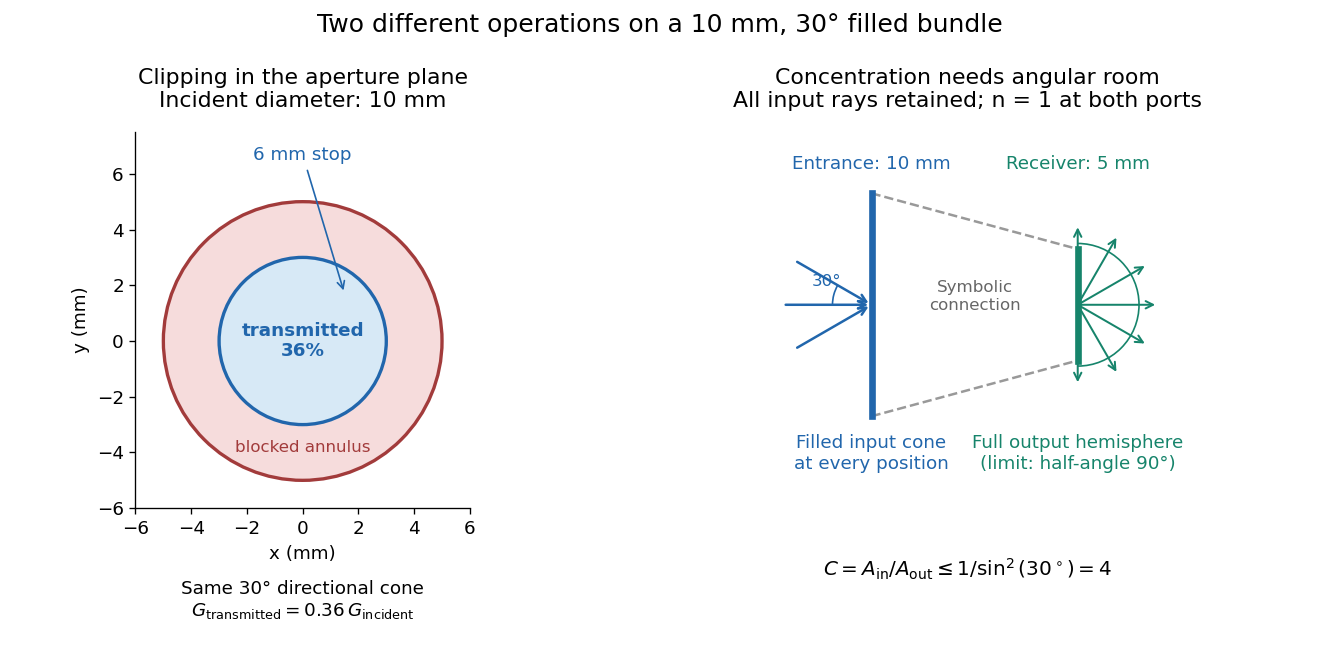
For the $30^{\circ }$ input cone with $n_{\mathrm{in}}=n_{\mathrm{out}}=1$, $C\le 4$: a $10\mathrm{mm}$ entrance cannot deliver the entire filled bundle to a circular receiver smaller than $5\mathrm{mm}$ in diameter. If the output half-angle is restricted to $60^{\circ }$, $C\le 3$ and the receiver diameter must be at least $10/\sqrt{3}\approx 5.7735\mathrm{mm}$. For a receiver medium with model refractive index $n_{\mathrm{out}}=1.5$, the full-hemisphere capacity bound instead gives $C\le 9$; that larger value also depends on transmitting the bundle into that medium.

Attempting $C=10$ in the air-to-air example forces rejection of some input. For the uniform radiance already specified, even filling the entire output hemisphere givesThe maximum mean irradiance gain remains $\eta C\le 4$. With nonuniform radiance, rejecting a given fraction of geometric etendue need not reject the same fraction of radiant flux.

These bounds use a filled extended-source bundle in passive reversible geometrical optics, comparing the same wavelength and the same radiation channels. An ideal optical point source does not fill that four-dimensional set. Diffraction, optical coherence, or coupling a Gaussian beam into an optical fiber require a physical optics calculation; the cone bound is not a universal guarantee for a single wave mode. Likewise, optical gain or fluorescence changes the propagation assumptions.

For a linear operator bounded from $L^{p_i}$ to $L^{q_i}$ with norms $M_i$, $i=0,1$, interpolate reciprocals by $1/p=(1-\theta )/p_0+\theta /p_1$ and $1/q=(1-\theta )/q_0+\theta /q_1$. The intermediate operator norm is at most $M_0^{1-\theta }{M}_1^{\theta }$. The complex interpolation proof first treats simple functions; completeness and continuity on the endpoint sum spaces identify the extension with the original operator. On finite counting spaces it also gives norm bounds between sequence spaces.

An open normal subgroup $N$ of a topological group is simultaneously open in its topology and invariant under conjugation. For a profinite group, the quotient $G/N$ is a finite discrete group: its cosets form a disjoint open cover, so compactness gives finitely many. Conversely the group homomorphism kernel of a continuous homomorphism to a finite discrete group is open and normal. Such subgroups form an identity-neighbourhood basis of every profinite group.

The Dedekind eta function modular transformation gives $F(e^{-t})\sim (t/2\pi {)}^{12}\exp (4{\pi }^2/t-t)$. The saddle-point approximation for coefficient extraction has $t_0=2\pi /\sqrt{p-1}$, phase $4\pi \sqrt{p-1}$ and curvature $(p-1{)}^{3/2}/\pi$. Its prefactor $t_0^{12}$ supplies $(p-1{)}^{-6}$ and the Gaussian width supplies $(p-1{)}^{-3/4}/\sqrt{2}$. This explains both the exponential growth and the power $-27/4$.

On $0\le \sigma \le \pi$, a coordinate with Neumann boundary conditions at both ends has a constant position, linear time zero mode and cosine oscillators. A coordinate with Dirichlet boundary conditions at both ends has a linear spatial interpolation between endpoint positions and sine oscillators, with no momentum zero mode. Both have integer frequencies. This differs from an ND boundary condition, which applies different conditions at the two ends of the same coordinate and gives half-integer frequencies.

An affine open cover of a scheme is an open cover by affine open subsets. Every scheme has such a cover by definition. A quasi-compact scheme has a finite affine open cover. Whether the intersections are affine is a further condition, supplied in particular by separatedness over an affine base.

A subcover of an open cover $\{U_i:i\in I\}$ of a subset $K$ is a selection of its members whose union still contains $K$. The selected open sets retain their original sizes; selecting a subcover does not mean replacing them by smaller open sets.

Use the Minkowski generating functional $Z=e^{iW}$, source $+J\varphi$, mean field $\phi =\delta W/\delta J$, and quantum effective action $\Gamma =W-\int J\phi$. Then $W^{(2)}=i{G}_2^c$, $W^{(3)}=-G_3^c$, and ${\Gamma }^{(2)}=-(W^{(2)}{)}^{-1}$. Differentiating this inverse gives ${\Gamma }^{(3)}=(W^{(2)}{)}^{-1\otimes 3}{W}^{(3)}=-i(G_2^c{)}^{-1\otimes 3}{G}_3^c$, with integration over the repeated spacetime arguments. Thus amputation of external propagators gives $i{\Gamma }^{(3)}$ in this convention. The full connected two-point functions, rather than bare propagators, perform the exact amputation.

Let $H$ be any antiderivative of the initial velocity, $H^{\prime }=g$. One choice of profiles isOpposite additive constants in $F$ and $G$ cancel, so the displacement is independent of the chosen antiderivative. Even for compact support of $g$, these separate profiles can approach nonzero constants; cancellation in their sum is essential to support widening for the wave equation.

For a short derivation, the characteristic coordinates $\xi =x-ct$, $\eta =x+ct$ give $u_{tt}-c^2{u}_{xx}=-4c^2{u}_{\xi \eta }$ by the chain rule. Thus $u=F(\xi )+G(\eta )$, and the Cauchy data imply $F+G=f$ and $-c{F}^{\prime }+c{G}^{\prime }=g$, giving the profiles above.

These characteristic curves are straight when wave speed $c$ is constant. A right-moving component is constant on $x-ct=s$, and a left-moving component on $x+ct=s$. The full superposition generally is not constant on either family, because the other component can vary along it. Their backwards intersections with the initial line select the endpoints used in D'Alembert's formula.

A conditional odds ratio can differ from the marginal odds ratio after averaging over a predictor, even without confounding. If conditional risks are $p_a(x)$, averaging gives ${\bar{p}}_a=\int p_a(x)dF(x)$, and odds of ${\bar{p}}_a$ are generally not averages of the conditional odds. Consequently a common conditional odds multiplier need not equal the marginal odds multiplier. However, if both groups use the same distribution $F$ and $p_1(x)>p_0(x)$ everywhere, then ${\bar{p}}_1>{\bar{p}}_0$ and the marginal odds ratio is still above one. Noncollapsibility alone cannot reverse a uniformly signed effect under an identical background distribution.

This range lies above both the Kolmogorov length scale and the scalar diffusion cutoff, but below the forcing scale. Molecular viscosity and scalar diffusion have negligible direct influence on transfer at those scales. The Obukhov-Corrsin theory predicts a two-thirds scalar structure function there.

For scalar diffusivity much smaller than kinematic viscosity, a scalar has structure below the Kolmogorov length scale while the velocity is smooth. The strain rate $s\sim (ϵ/\nu {)}^{1/2}$ transfers scalar variance, giving $d{S}_C/dr\sim {ϵ}_c/(sr)$. Integration produces a logarithm plus an additive matching constant.

For scalar diffusivity much larger than kinematic viscosity, scalar diffusion dominates at lengths between the Kolmogorov and scalar cutoff scales. The velocity may still have inertial-range variations, but the scalar is smooth to leading order. The leading isotropic scalar structure function is quadratic, with coefficient fixed by the mean-square gradient and the scalar dissipation rate, rather than by a continuing inertial-convective two-thirds law.

A cross-sectional study measures different individuals during one observation period. Differences between ages can reflect confounding or birth-cohort differences as well as changes within individuals; a longitudinal study is needed to measure the latter directly.