
Empirical likelihood with mixed censoring Created 2026-10-14 Updated 2026-11-05
For independent event times with survivor function , an exact event at contributes mass , a right-censored observation at contributes , and an interval-censored observation contributes . Multiplying these factors gives the event-time likelihood when the observation mechanism is noninformative. Maximizing over nonincreasing right-continuous survivor functions gives a nonparametric maximum-likelihood estimator rather than requiring a parametric density.
Interior second-derivative estimate for the Poisson equation Created 2026-10-14 Updated 2026-10-25
If and weakly, then . Test the weak equation with , move the first difference quotient onto , and bound the remaining quotient on the forcing side by the first derivative of . Young inequality absorbs the localized second derivatives. Uniform bounds in , together with the Sobolev characterization by bounded difference quotients, give the assertion without differentiating . The constant depends only on dimension and the positive distance from to the boundary of .
// Target: geometry-and-topology.bigb
Lemniscatic integral 2026-10-14
Choose the holomorphic square root equal to one at zero on the unit disc. The resulting elliptic integral maps that disc conformally onto the square with vertices , where . For the inverse Cayley transform between the half-plane and disk , the square of the derivative of , with , is . Thus the two square maps differ by an affine change of coordinate.
Ellipse perimeter expansion near a circle 2026-10-14
For an ellipse with semiaxes , the perimeter integral has integrand . The uniformly convergent binomial series near permits termwise integration. Integrals of and over a full period give the displayed first corrections. The same coefficients follow from the Frobenius method for the transformed perimeter equation.
Semi-major and semi-minor axes Created 2026-10-14 Updated 2026-10-20
The semi-major and semi-minor axes are the larger and smaller half-axis lengths of an ellipse. In principal-axis coordinates the ellipse has equation with . The same terminology is used for a hyperbola , where is half its transverse axis and half its conjugate axis. Orbital semiaxes apply these geometric quantities to conic sections.
In the space of infinite subsets of the natural numbers, the families are clopen sets in the ordinary topology on infinite subsets and thus in the finer Ellentuck topology. Their union is . Every basic Ellentuck topology neighborhood of contains for some sufficiently large , so this union is not a closed set.
Cone on an infinite coinfinite ground set 2026-10-14
For an infinite coinfinite set , let in the space of infinite subsets of the natural numbers. This cone is a nonempty clopen set in the Ellentuck topology, because it is the basic neighbourhood , and any has a finite initial segment containing a point outside and hence a basic neighbourhood disjoint from .
The cone is a closed set with empty interior in the ordinary topology on infinite subsets: membership of a point outside witnesses its complement as an open set, while every ordinary finite-stem neighbourhood can be extended by an arbitrarily large point outside . Thus is an ordinary nowhere dense set, but it is neither ordinary open nor Ellentuck nowhere dense. It provides both distinctions between these two topologies.
Ellentuck Borel sets are completely Ramsey 2026-10-14
Every Borel set for the Ellentuck topology is completely Ramsey. First, an acceptance-and-rejection fusion makes every open set homogeneous after thinning the infinite reservoir while keeping its finite stem. Every nowhere-dense set is consequently completely Ramsey-null, and a fusion handling all subsets of each finite selected prefix shows that countable unions of such null sets remain null. Finally, sets differing from an open set by a meagre set form a sigma-algebra containing the open sets. Thus every Borel set has the required stem-preserving homogeneous refinement.
Taylor identity for quasi-geostrophic flux 2026-10-14
For zonal averages, , , and , with depending only on height, define and . Integrating zonal derivatives by parts gives . This identity is exact within quasi-geostrophic potential vorticity, without assuming small disturbance amplitudes. Periodicity or appropriate vanishing zonal boundary terms is essential.
Electromagnetic charge matrix of electroweak gauge fields Created 2026-10-14 Updated 2026-11-05
In the basis with gauge transformations and , the non-Abelian connection transforms by conjugation. The Lie brackets and give , , with neutral . Thus gives the displayed Hermitian matrix. The fields transform as , while both neutral combinations are uncharged. This separates the Adjoint representation on the gauge fields from the doublet charge matrix on the Higgs field.
Reduced electron magnetohydrodynamics Created 2026-10-14 Updated 2026-10-20
With , define and to leading order. Let , where . The leading electron velocities are and . Substitution into frozen-in induction yieldsLinearization gives , agreeing with the full EMHD relation to leading anisotropic order. If varies along the guide field, an order-smaller perpendicular gradient correction restores exact solenoidality; the two-field representation is not an exact decomposition at arbitrary anisotropy.
Whistler wave Created 2026-10-14 Updated 2026-11-05
In the inertia-free, constant-density electron magnetohydrodynamics model with uniform guide field , a transverse magnetic plane wave obeys . The helicity decomposition of a transverse Fourier mode gives the displayed dispersive branches with opposite circular polarizations. This electron-current mode is called a whistler wave; see Lyutikov's analysis of electron magnetohydrodynamics. Its pressure-free induction equation should not be identified with a general kinetic Alfvén model.
Weak electron-magnetohydrodynamic cascade 2026-10-14
For , the weak wave cascade estimate gives . Constant energy flux yields the displayed amplitude. An additionally isotropic local cascade has and shell-integrated magnetic energy spectrum . These statements are phenomenological consequences of the chosen locality and decorrelation assumptions.
Critical balance sets , hence . A local strong cascade with constant energy flux has , giving the displayed exponents and perpendicular magnetic energy spectrum . The anisotropy becomes stronger towards small perpendicular scales.
Electrochemical gradient Created 2026-10-14 Updated 2026-10-25
An electrochemical gradient combines spatial changes in chemical potential and electric potential for a charged species. Passive transport proceeds downhill in electrochemical potential when an appropriate route is available; a concentration difference alone does not determine the direction for an ion.
Electrical conductance 2026-10-14
For an ohmic element with finite nonzero electrical resistance , its electrical conductance is : an electric potential difference drives electric current . Greater positive electrical conductance means a greater electric current for the same positive electric potential difference. Electrical conductivity is instead a bulk material coefficient relating current density to electric field.
Electrical reactance bench measurement 2026-10-14
The motivating observation is a pair of sinusoids on an oscilloscope: changing frequency changes both their relative amplitudes and their phase difference. Gary Tuttle's EE 201 laboratory uses resistor voltage as the current-phase reference, compares predictions with readings at several frequencies, and explicitly asks students to measure component values and account for coil electrical resistance. The following bench arrangement applies that method to a series RLC circuit; its component values and illustrated traces are our own toy example. [ref]
https://gtuttle.net/circuits/lab/ac_circuits_1.pdf. Gary Tuttle, EE 201 Lab 9: AC circuits, especially the notes and RC/RL measurements
.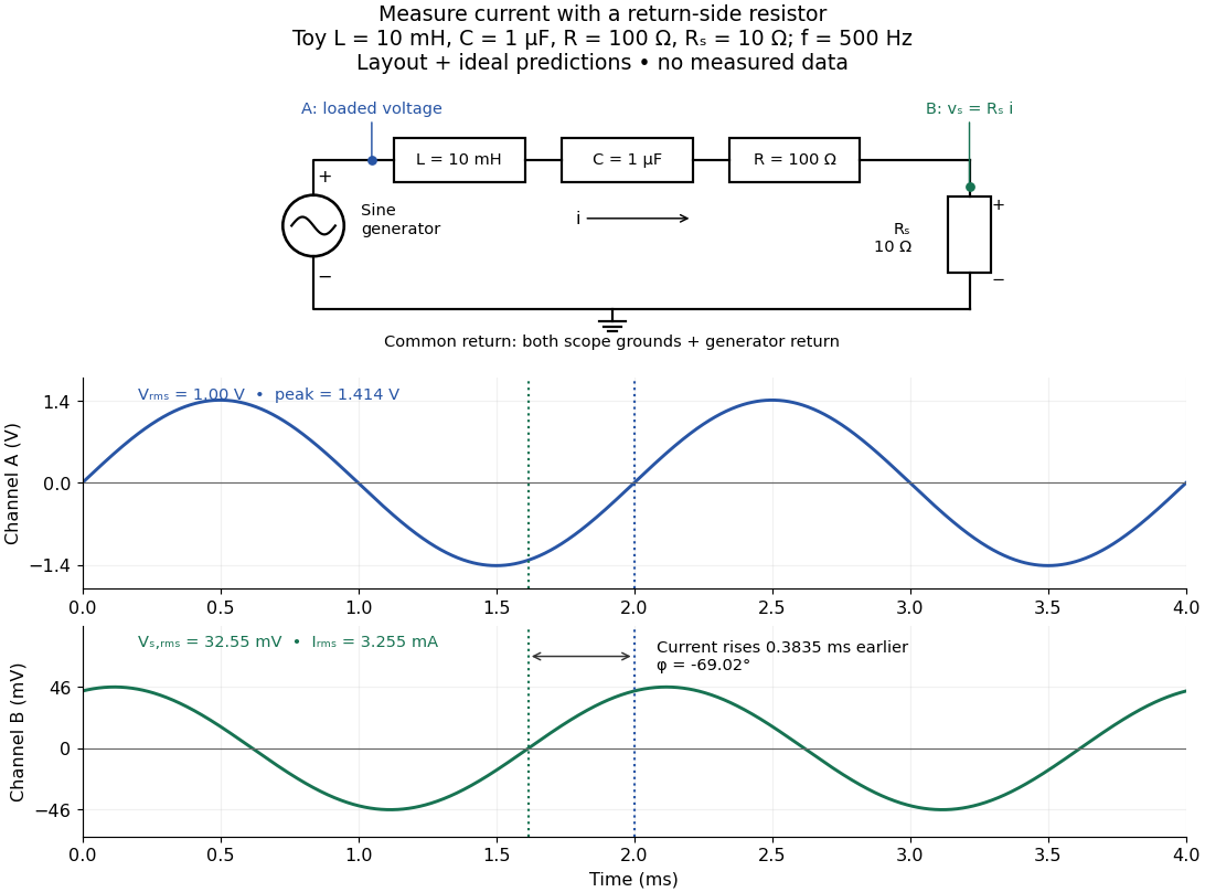
Toy AC bench arrangement and predicted voltage/current timing
. Top: a sine generator drives ideal , , , and current-sensing in series. Channel A measures loaded terminal voltage; channel B measures relative to the common return. Bottom: calculated separate voltage traces at and terminal , not an oscilloscope recording or measured data. The rising zero of channel B occurs earlier: and predicted . The two trace axes have different voltage scales. Details.
Connect a low-voltage sine generator to a series chain ending in a known sensing resistor at the common return. Use a resistor whose unwanted inductance is negligible over the chosen frequency range. An oscilloscope displays voltage against time: channel A reads the loaded voltage across the whole chain, and channel B reads the voltage across . Both channel ground connections and the generator return meet at that same node. Ordinary bench oscilloscope grounds are electrically common; attaching one to an intermediate circuit node would change the circuit. A separate floating component voltage needs a suitable differential measurement, rather than moving a ground clip. [ref]
https://www.tek.com/en/documents/technical-brief/floating-oscilloscope-measurements-and-operator-protection. Tektronix, Floating Oscilloscope Measurements and Operator Protection: ground-referenced inputs
.After the free transient decays, record frequency , period , both voltage amplitudes, and matched rising zero-crossing times . Check that the traces are sinusoidal. Define on the branch . With negligible probe loading and negligible sensing-resistor electrical reactance, , so channel B is the electric current reference, and in the reactance phase conventionA later current crossing gives , hence positive electrical reactance; an earlier crossing gives negative electrical reactance. Use the same amplitude convention for both channels. An amplitude-only ratio recovers , so it cannot distinguish the two signs: timing supplies the missing information. The formulas follow from and the chosen terminal orientation.
Begin with a known resistor replacing the reactive chain: its expected phase difference is approximately zero, testing channel polarity and relative delay. Measure the same signal with both channels to establish the instrumental delay baseline, then exchange probes to check that a phase offset does not belong to one channel. Next test an inductor and a capacitor separately with : after subtracting from the inferred real part, expect approximately and , respectively. Finally combine and sweep through the predicted resonance. These are proposed controls and consequences of the model, not reported observations.
For the toy series RLC circuit, the prediction at is , , , and . At , and . Near the model predicts zero phase difference and . Keep actual loaded fixed or normalize by it at each frequency; the generator's display alone does not establish that voltage. The sensing resistor is part of the total and therefore changes the predicted peak electric current.
Real components add unintended electrical impedance: coil wire has electrical resistance, nearby turns add capacitance, and capacitor leads add inductance. These effects can produce a component's own resonance, beyond which the ideal or approximation fails. Work in a range where that approximation is adequate, measure coil wire electrical resistance, and compare the inferred with the sensing resistor, intended resistor, and component losses. A measured nonzero real part is evidence of loss in the assembly, not negative or positive electrical reactance becoming heat. [ref]
https://www.keysight.com.cn/cn/zh/assets/7018-06840/application-notes/5950-3000.pdf. Keysight, Impedance Measurement Handbook, §§1.5.1 and 5.2.1: component frequency response and parasitic elements
; [ref]https://gtuttle.net/circuits/lab/ac_circuits_1.pdf. Tuttle, EE 201 Lab 9: parasitic coil series resistance
.The probes also add electrical resistance and capacitance to the measured nodes; their loading becomes more important as frequency increases. Use compensated probes with known input electrical impedance and short ground connections, and repeat with a smaller drive voltage to test whether the inferred depends on amplitude. [ref]
https://www.tek.com/en/documents/application-note/how-oscilloscope-probes-affect-your-measurement. Tektronix, How Oscilloscope Probes Affect Your Measurement: resistive and capacitive loading
. Record actual voltage and phase readings separately from calculated predictions, with component tolerances and timing uncertainty. A phase error alone produces approximately , so near zero electrical reactance, a small delay can imitate a small residual . Agreement within stated uncertainties tests the model; the smooth toy curves establish no experimental accuracy. Reactance phase convention 2026-10-14
Use complex amplitudes only for signals at one common positive angular frequency . Define the real terminal voltage and electric current byThe complex amplitudes here use peak magnitudes; both can instead use root mean square magnitudes without changing their ratio. Choose positive electric current entering the terminal assigned positive voltage, so is absorbed power. For an ideal linear inductor and capacitor, their terminal laws and giveThe derivative multiplies a complex amplitude by : this single algebraic step explains both signs. Taking as a reference gives and for the sinusoidal response. Thus inductor voltage leads electric current by , while capacitor voltage lags electric current by . A constant offset or a free transient is outside this single-frequency representation. [ref]
https://www.feynmanlectures.caltech.edu/II_22.html#Ch22-S1. Feynman, Leighton and Sands, II.22.1: complex sinusoidal representation and component impedances
.With the alternative convention, the same real signals use conjugated complex amplitudes and , . Their physical leads and lags stay the same; the sign of changes. Also, some textbooks call the positive magnitude the capacitive reactance and write the series expression as . This article consistently uses signed and hence . [ref]
https://openstax.org/books/university-physics-volume-2/pages/15-2-simple-ac-circuits. Ling, Moebs and Sanny, University Physics 2, §15.2: positive capacitive-reactance magnitude and quarter-cycle phase relations
. Rayleigh wave 2026-10-14
A Rayleigh wave propagates along a stress-free boundary of an isotropic elastic half-space and decays into its interior. It combines an evanescent longitudinal wave with an evanescent vertically polarized shear wave. If its speed is , the decay factors are and . Vanishing shear and normal traction gives the displayed determinant condition.
Love wave 2026-10-14
A Love wave is a horizontally polarized shear wave trapped in a slower elastic surface layer above a faster elastic half-space. Zero shear traction at the free surface, displacement continuity and traction continuity at the interface produce its dispersion relation. A trapped mode has phase speed between the two shear speeds and decays exponentially into the half-space.
There are unlisted articles, also show them or only show them.