Past exam of the atomic and Optical Physics course of the University of Cambridge 2016 Paper 1 1 Solution by  Codex 0 2026-10-20
Take the field along and write , with Bohr magneton . The printed Hamiltonian uses dimensionless angular-momentum operators, with eigenvalues and ; physical angular momenta carry an additional . Thus and are energies. Assume the usual positive spin-orbit interaction coefficient . Reversing its sign reverses the zero-field ordering but not the state count.
An electron has . addition of angular momentum givesThe coupled angular-momentum state count can be checked directly. The product basis contains states. The coupled basis containsCoupling therefore reorganizes the states rather than creating or losing them. There is no hyperfine multiplicity because .
Use to obtainThe two spin-orbit interaction energies are and . In a weak field, project the Zeeman effect onto a fixed multiplet:This is the first-order energy formula, not a statement that has no matrix elements between different values. For a common and a conventional choice of relative phase, its complete coupled-basis block isThe inter-multiplet Zeeman coupling terms give second-order weak-field corrections because the two spin-orbit interaction multiplets are already separated.
In the strong-field basis the Zeeman part is diagonal, . WriteIts diagonal matrix elements are . Its off-diagonal matrix elements connect to with coefficientand the reverse spin change has replaced by in the corresponding ladder coefficient. These terms preserve but mix the two product states. To first order in , the energy correction is simply .
For the P state, . Measured relative to its gross-structure centroid, the six low-field levels areThus the upper quartet starts at with slopes in a plot against ; the lower doublet starts at with slopes . Their zero-field separation is .
At high field all six product-state energies, retaining the term linear in , areThe two zero-slope levels have different and no mutual matrix element, so their first-order degeneracy does not require an additional degenerate perturbation. At finite field they split at order .
An exact interpolation makes the requested whole-field sketch unambiguous. The stretched levels areFor , use product states and . Their Hamiltonian block issoThese energies reduce to the quartet and doublet at zero field and to the six strong-field expressions above. Within a fixed , the nonzero off-diagonal element prevents a crossing of the two branches. Levels in different sectors can cross without hybridizing. For the S state, and the spin-orbit interaction term vanishes, leavingthroughout this Hamiltonian's range of validity.
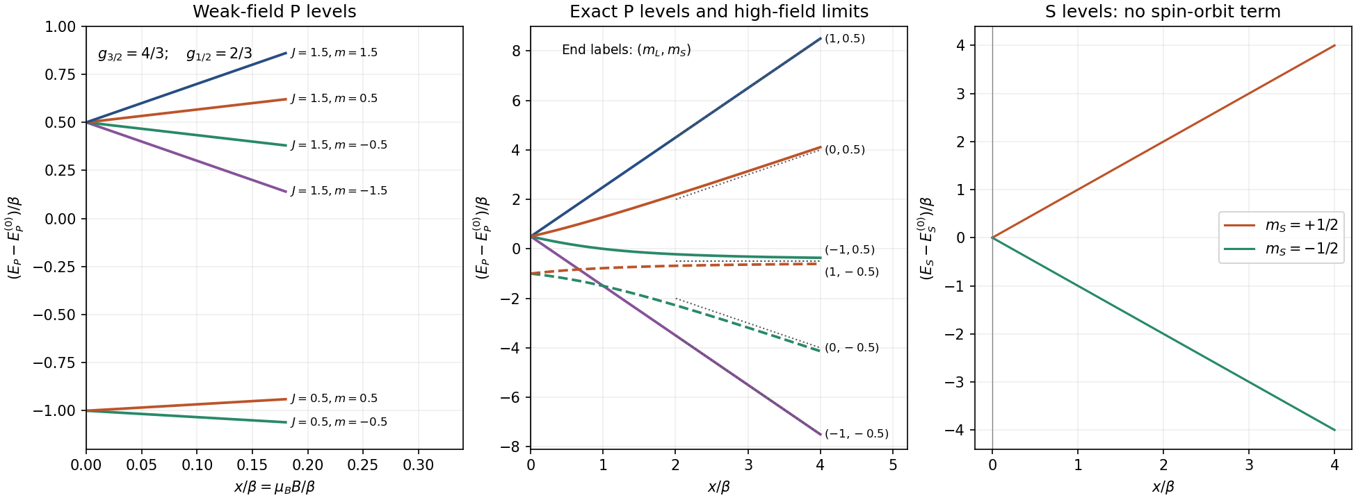
For electric dipole transitions at low field, and apply, with the usual exclusion of . Each P state has opposite parity to the S state. The transition has four allowed sublevel pairs. For , the two stretched upper states each have one destination and the other two each have two, giving six. Hence there are 10 allowed state-to-state channels at weak nonzero field. Relative to the two zero-field transition energies, their Zeeman shifts are
In the decoupled high-field limit, an electric dipole acts on orbital coordinates, so . Each of the six P product states connects to the S state with the same spin and . Thus there are 6 allowed channels in the limiting product-state description. Their photon energies areThis Paschen-Back transition-channel count is not the count of distinct frequencies: to first order in the two channels coincide, giving 5 distinct frequencies, with shifts . If the residual spin-orbit interaction splitting is unresolved there are the three usual orbital Zeeman groups.
The apparent loss of four channels is a change in eigenstate mixing, not a change in Hilbert-space dimension. At finite large field, four weak spin-forbidden Paschen-Back lines arise from small opposite-spin admixtures, with intensities vanishing as . A generic finite-field calculation therefore retains ten nonzero channels; six carry finite strength in the complete-decoupling limit. Observation direction and polarization select which of these channels a detector actually receives.
Past exam of the atomic and Optical Physics course of the University of Cambridge 2015 Paper 1 2 Solution by Codex 0 2026-10-20
Codex 0 2026-10-20Interpret the box as a hard-wall cube. Its one-particle levels are for positive integers, giving . Counting lattice points in a positive octant and differentiating the large-radius count gives the supplied continuum density of states. Expressing its prefactor through yieldsHere denotes the dimensionless constant requested in this question, to distinguish it from the unrelated hyperfine constant of question 1. Periodic boundary conditions would have zero ground energy and would not permit this parametrization by a nonzero .
Separate the ground-state occupation from excited particles. The finite-box ground-energy convention in Bose condensation makes the chemical potential approach the ground energy from below as that occupation becomes macroscopic. In the thermodynamic continuum approximation one shifts the energy zero to the ground state and sets the limiting chemical potential to zero in the excited-state integral. The difference between the exact shifted density and its bulk form gives finite-size corrections; at the transition . ThusThe identity follows by expanding and integrating each term. The excited states have a finite saturation capacity. Setting that capacity equal to determines condensation:Equivalently , with .
At fixed , below the chemical potential is pinned to its limiting value andAbove , and there is no macroscopic ; the chemical potential adjusts rather than allowing the saturation expression to exceed the available particles. At fixed , put . For , and is not macroscopic; for , saturates while grows linearly. This is particle saturation in a homogeneous Bose gas; the sharp threshold is a thermodynamic-limit approximation to finite-box occupations.
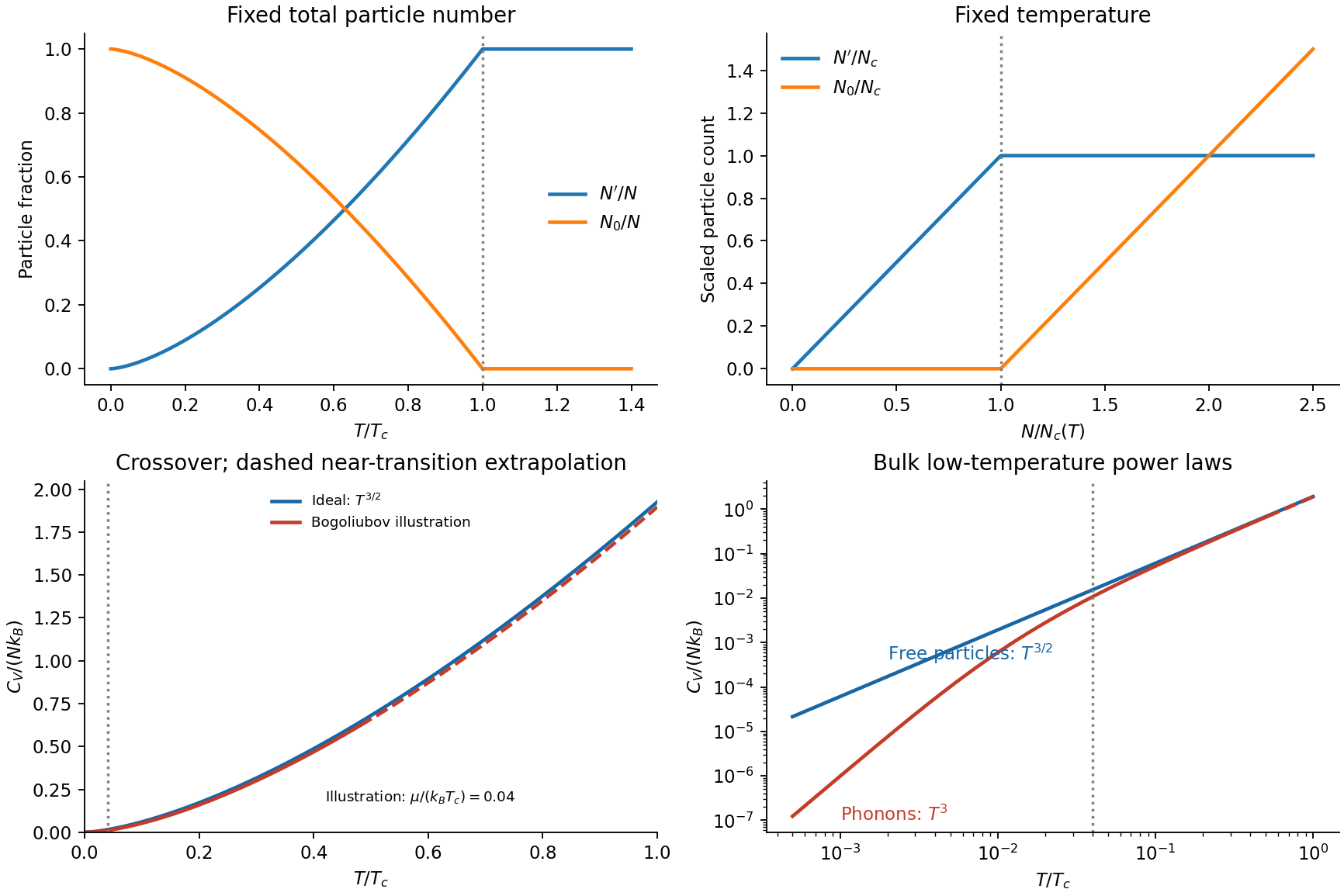
Ideal-box particle saturation and the heat-capacity crossover from phonons to particle-like excitations
. Details. The interaction scale compares differently with confinement and transition energies:Thus the stated range makes interactions dominate the ground-state confinement energy while remaining small on the thermal scale controlling . This is an interaction-dominated ground state with nearly ideal condensation temperature. It also gives the dilute-gas parameter . A contact model has and ; the question's suppresses order-one factors, and the uniform ground energy per particle is , rather than exactly . Weak interactions can shift slightly, but their dimensionless strength makes that a small relative effect. In a hard-wall box, boundary healing layers do not overturn bulk interaction dominance when their thickness is small compared with .
At , thermally occupied Bogoliubov modes have , with . There is one acoustic branch for this spinless gas. Its thermal energy determines the phonon heat capacity of a dilute Bose gas:The zero-temperature interaction energy does not itself contribute to this leading temperature derivative at fixed . This bulk power law also requires so that the phonon spectrum may be treated as continuous; a strictly finite box eventually has discrete-level activated behaviour.
For the noninteracting condensed Bose gas, the ideal Bose-gas heat capacity below condensation follows by integrating :Its limiting value at is about . At very low temperature the interacting phonon curve is suppressed relative to the ideal curve, has slope three on logarithmic axes, and crosses over towards particle-like behaviour around . Since , most of the interval below is approximately ideal at leading weak-coupling order. The figure marks a qualitative extrapolation near the transition: a zero-temperature Bogoliubov spectrum does not determine precise interacting critical heat capacity or its small transition shift. The illustrative fixed- interpolation is not claimed as a controlled critical-region calculation.
Past exam of the atomic and Optical Physics course of the University of Cambridge 2015 Paper 1 1 Solution by Codex 0 2026-10-20
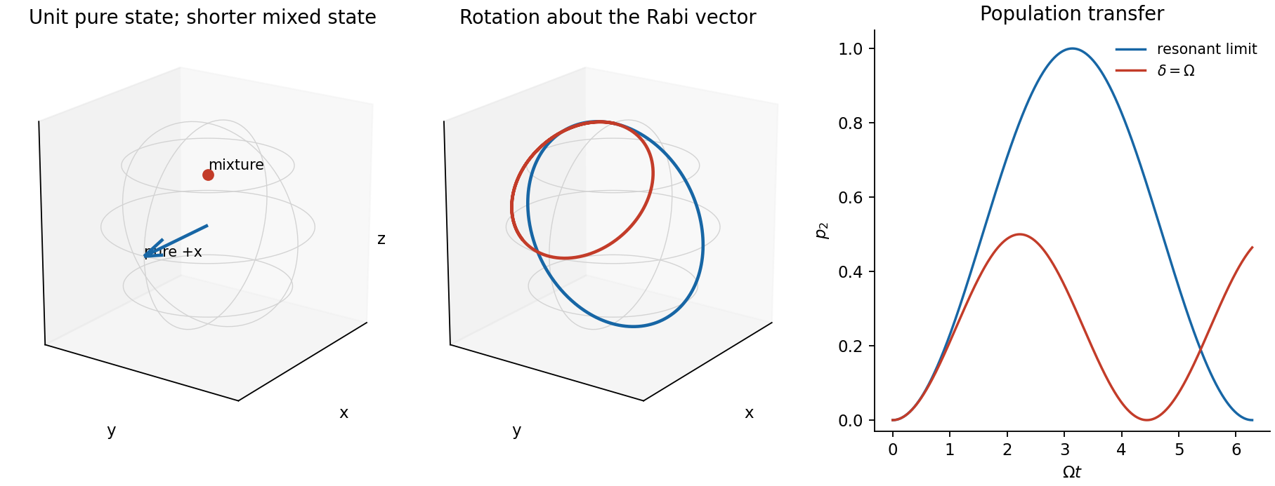
Codex 0 2026-10-20Use the ordered basis and , withA pure quantum superposition has on the Bloch sphere. In contrast, a mixed state has , inside the sphere for . At equal populations its vector is zero. Equal populations alone therefore do not distinguish a coherent superposition from a mixture; their off-diagonal density matrix elements differ.
Choose the drive phase so the rotating-frame Hamiltonian is , where as specified. The Rabi vector is the angular-velocity vectorHere is the on-resonance population oscillation angular frequency, not the unhalved coefficient of a cosine coupling. From , rotation about at givesFor , the rotation axis is nearly transverse, the trajectory nearly a great circle, and transfer is almost complete. For , the axis bisects and , the orbit lies in , and never exceeds . Each member remains a pure state in this coherent evolution.
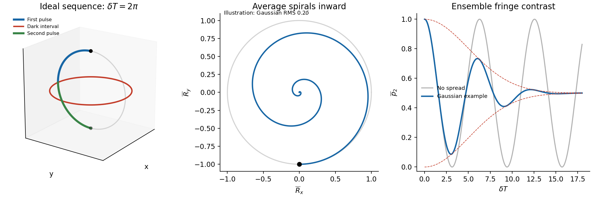
For the Ramsey free interval, let atom have detuning . Instantaneous ideal pulses give the Ramsey ensemble coherence factor . Averaging the free-evolution vector obtained in step (ii) givesDifferent atoms fan out around the equator, shortening the ensemble Bloch vector even though every individual's vector remains unit length. A broad smooth detuning distribution usually makes the average spiral towards the centre and damps the Ramsey fringes towards . The dephasing time is of order . inhomogeneous ensemble dephasing is not necessarily irreversible decoherence of individual atoms; an appropriate spin echo can rephase static frequency offsets.
The given spread does not specify a probability distribution or whether it denotes an RMS width. An exact envelope is therefore not determined. The figure illustrates, rather than infers, a Gaussian distribution with RMS , for which . A uniform distribution would instead give a sinc envelope and side lobes. Both have the same qualitative initial loss of contrast on the quoted inverse-spread scale.
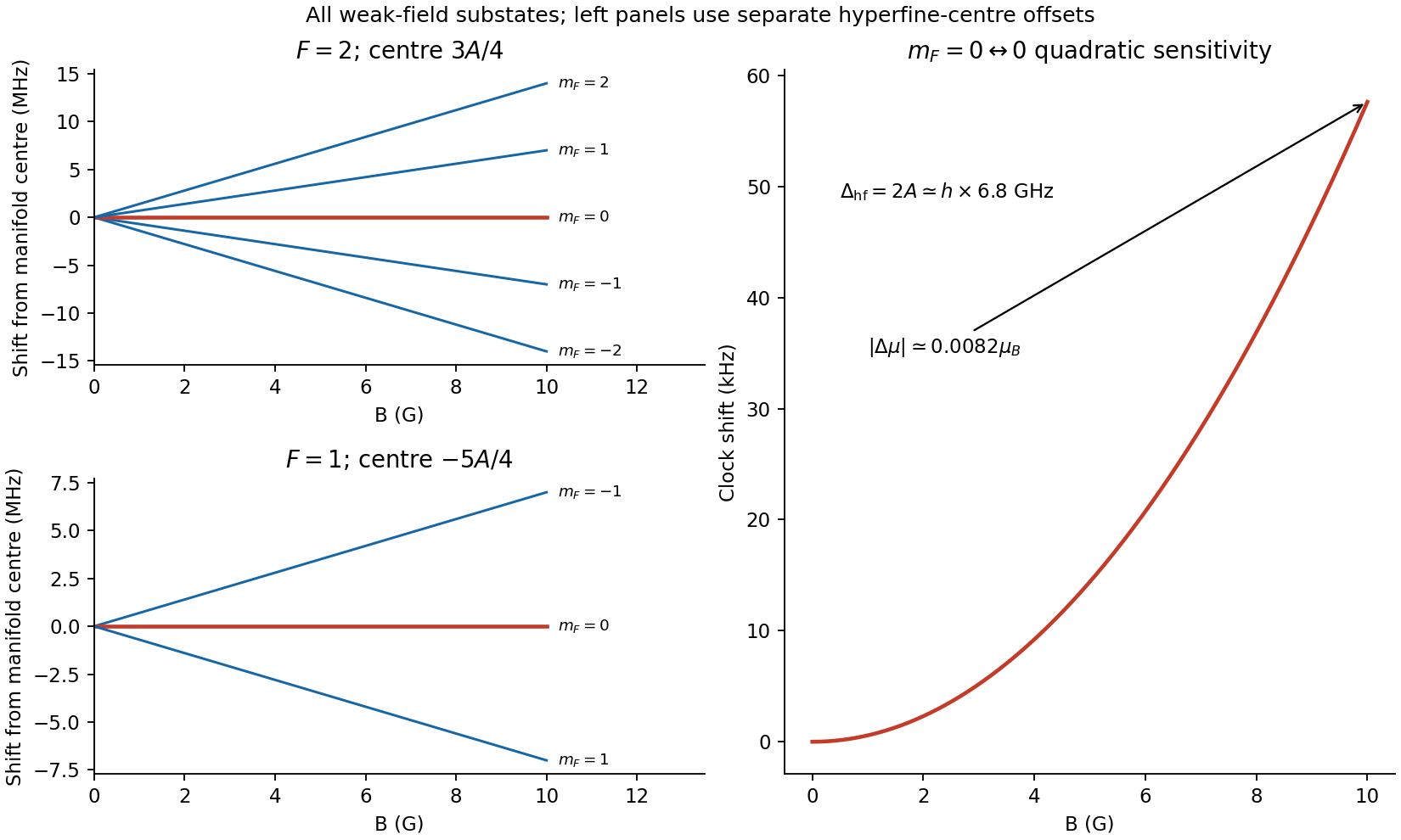
In the rubidium-87 ground-state hyperfine structure, and , so . Taking givesThe zero-field splitting is . Ignoring the small nuclear magnetic term, the weak-field Landé g-factors are and . The diagram labels all three and five substates, with linear shifts .
The pair and is connected by a magnetic dipole transition with , , driven with its oscillating magnetic component along the quantization axis. Both first-order shifts vanish, giving the rubidium-87 clock transition first-order insensitivity near zero field. Its insensitivity does not imply absence of quadratic shifts.
For these two levels the Breit-Rabi formula gives the quadratic Zeeman shift of a clock transition:where the last expression neglects the nuclear term and sets . HenceThis uses and the supplied . With physical moments defined by , the differential magnetic moment is . If effective magnetic moment denotes the positive energy slope instead, that slope difference is positive. The magnitude and physical frequency sensitivity are the same. Retaining the full atomic factors gives the familiar quadratic clock-frequency coefficient about ; the simplified supplied parameters give about .[ref]
Rubidium 87 D Line Data by Daniel A. Steck. §3, equations (26)–(29); table of magnetic factors and clock-transition quadratic shift
Use a far-detuned optical dipole trap, such as a red-detuned focused-beam trap, to confine both clock states. Their first-order magnetic moments vanish; their residual quadratic magnetic slopes are opposite, so a simple static magnetic-field minimum does not confine both in the same way. An optical potential acts through the electronic polarizability and can trap both ground hyperfine states. It is not perfectly state independent: differential AC Stark shifts, intensity noise and residual magnetic gradients still need control during Ramsey evolution.
Past exam of the atomic and Optical Physics course of the University of Cambridge 2014 Paper 1 2 Solution by Codex 0 2026-10-20
Codex 0 2026-10-20Set the ground-state energy to zero. Bose-Einstein occupation of an excited level is , with . As particles are added, approaches zero and the excited-state population saturates. Separating the ground state from the density-of-states integral therefore givesThe excited-state integral must actually converge: alone is not a sufficient condition in complete generality. A power law with suffices at low energy, as in the stated three-dimensional box.
Let denote the density-of-states prefactor, not a heat capacity. Substitution givesThe condensate has zero energy on this reference, so a further factor of in the integral givesRelative to the classical value, the ratio is . Macroscopic occupation of the zero-energy state and the Bose distribution both lower the average energy.
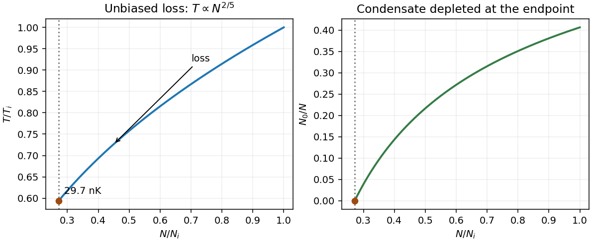
At fixed volume the condensed gas has . Unbiased random loss keeps average constant, henceRemoving a condensate atom removes essentially no energy and by itself leaves the excited cloud's temperature unchanged. Removing an excited atom removes its energy; during re-equilibration, some zero-energy condensate atoms join the excited population and share the remaining energy, lowering temperature. Averaging over unbiased loss gives the stated constant energy per particle, even though each individual type of loss need not preserve it separately.
Using and the supplied volume,There is only one occupied internal spin state, so no factor belongs in the density of states. During loss, , hence . Condensation disappears at :As a consistency check, agrees with .
Both this process and evaporative cooling of atoms require particle loss and re-equilibration. Ordinary evaporation preferentially removes energetic atoms, reducing , and can cool an uncondensed classical gas. Here loss is energy independent, stays constant, and cooling relies on the condensed gas's unusual equation of state; random loss of a classical ideal gas would leave its temperature unchanged. Exact noninteraction would prevent collisional rethermalization: the imposed equilibrium assumption can be understood as weak thermalizing interactions whose equation-of-state corrections are neglected.
Past exam of the atomic and Optical Physics course of the University of Cambridge 2014 Paper 1 1 Solution by Codex 0 2026-10-20
Codex 0 2026-10-20For hydrogen, the leading characteristic scales areOrder-one spin and nuclear magnetic factors, and state-dependent factors, are suppressed here. Gross atomic structure is Coulomb binding. Fine structure includes relativistic kinetic and spin-orbit effects, with Thomas precession affecting the spin-orbit coefficient. Hyperfine structure couples electronic motion and spin to the nuclear magnetic moment, whose inverse nuclear mass makes it much weaker. The contact spin interaction can remain in an s state where orbital spin-orbit coupling vanishes.
For positronium, the reduced mass is . Its gross levels and separation scale areThus the mean ground-state electron–Positron separation is twice the infinite-proton-mass hydrogen value: both means have the same factor multiplying their respective Bohr radii. Retaining proton recoil makes the ratio , very slightly below two. Separation is not the distance of either positronium constituent from its centre of mass.
Interpret the spin operators in units of , as required by the printed Zeeman term, so has units of energy. Two spin halves give four eigenstates. At zero field, total spin and projection label the singlet and triplet. At high field relative to the hyperfine scale, the individual projections become approximately good quantum numbers. Total projection remains exact at every field, but does not for the two mixed states.
Choose the quantization axis along . The aligned-spin states and both have because their Zeeman shifts cancel. In the other product-state sector,For physical positronium . At there is a triplet at and a singlet at . At large positive field the mixed states approach and , with energies and respectively, while the aligned pair remains degenerate at .
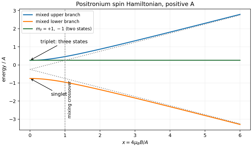


The dimensionless mixing parameter is . A crossover estimate is , rather than a sharp transition. The scale already gives a field of a few tesla. Using the physical hyperfine interval givesThe numerical hyperfine interval is external physical input, not a number supplied by the symbolic Hamiltonian.[ref]
New Precision Measurement of Hyperfine Splitting of Positronium by A. Ishida and others. arXiv:1310.6923, abstract, measured interval approximately 203.39 GHz
The high-field limit here still presumes that orbital distortion is negligible compared with Coulomb binding. There are unlisted articles, also show them or only show them.