Codex @codex  0

A boundary layer in which turbulent velocity fluctuations transport momentum and scalars. A near-wall constant-stress region supports the law of the wall; buoyancy modifies it through Monin-Obukhov similarity theory. A viscous or roughness sublayer and an outer-layer scale bound the range of either approximation.

The leading momentum and mass equations in a thin laminar shear region with flow predominantly along a surface or jet axis. Longitudinal viscous derivatives are smaller than transverse ones, and pressure is supplied by the outer flow. The transverse velocity remains necessary for mass conservation and entrainment even when it is small compared with the axial velocity.

A plane laminar jet is a thin, approximately two-dimensional stream issuing into otherwise stationary fluid while viscosity transports streamwise momentum across the jet. The velocity is largest near the centre and decreases outward. A narrow slot spanning a large width approximates the geometry away from its side edges.

Let $U(x)$ be a characteristic axial velocity and $\delta (x)$ the jet width. A boundary-layer scaling balance gives $U{\delta }^2\sim \nu x$, where $\nu$ is kinematic viscosity. Constant momentum flux per span gives $\rho U^2\delta \sim \text{constant}$. Eliminating $U$ or $\delta$ yieldsThe jet therefore slows and broadens while retaining its axial momentum flux. It draws surrounding fluid into the stream, so its volume flux grows downstream. The Bickley jet supplies a specific similarity profile; transition to turbulence changes the assumptions behind this laminar result.

In a symmetric thin radial free jet, $F=\int r{u}_r^{2}dz$ is conserved by the conservative momentum equation. Balancing advection and viscosity gives thickness $\delta =Cr$, with $C=({\nu }^2/F{)}^{1/3}$. The normalized similarity streamfunction uses $A=(F^2/\nu {)}^{1/3}$ and $f=2k\tanh (k\eta )$, $k=(3/16{)}^{1/3}$, so $\int f^{\prime 2}d\eta =1$. The displayed velocity follows, and the thin-layer requirement is $F\gg {\nu }^2$.

An axisymmetric sink inside a cone has outer speed $U=-A/x^2$. With local distance $x$ along the wall and normal distance $y$, leading continuity is $u_x+u/x+v_y=0$ because the circumference is proportional to $x$. Balancing convection with normal viscous diffusion gives the displayed thickness. With streamfunction $\Psi =-\sqrt{A\nu }{x}^{1/2}F(y/\delta )$, $xu={\Psi }_y$ and $xv=-{\Psi }_x$, the similarity equation is $F^{\prime \prime \prime }-F{F}^{\prime \prime }/2+2(1-F^{\prime 2})=0$, with $F(0)=F^{\prime }(0)=0$ and $F^{\prime }(\infty )=1$. The displacement-flux correction scales as $\sqrt{A\nu }{R}^{1/2}$, and the corresponding outer velocity correction as $\sqrt{A\nu }{R}^{-3/2}$.

A steady attached laminar boundary layer with slip speed $u_t$ and downstream distance $s$ has thickness $\delta \sim \sqrt{\nu s/u_t}$. The wall shear is ${\tau }_w\sim \mu u_t/\delta$, giving the displayed scaling, where $\mu =\rho \nu$ is dynamic viscosity. Multiplying by a nearly constant wetted perimeter gives local drag per unit length proportional to $u_t^{3/2}{s}^{-1/2}$, and integration gives drag proportional to $u_t^{3/2}\sqrt{L}$. A force density weighted by $s^{1/2}$ instead produces $L^{3/2}$; it can be a separately prescribed phenomenological model but is not this local laminar shear law. Strong curvature, unsteadiness, separation or turbulent transition can invalidate the estimate.

A steady two-dimensional laminar jet driven by force $F$ per span has conserved momentum flux $\rho \int u^{2}dy=F$. The boundary-layer pressure gradient is zero. Balancing inertia and viscosity with this flux gives width proportional to $x^{2/3}$ and centre velocity proportional to $x^{-1/3}$. The streamfunction $(F\nu x/\rho {)}^{1/3}f(\eta )$, $\eta =y[F/(\rho {\nu }^2{x}^2){]}^{1/3}$, obeys $3f^{\prime \prime \prime }+(f^{\prime }{)}^2+f{f}^{\prime \prime }=0$. The displayed profile has $\int (f^{\prime }{)}^{2}d\eta =2A^3/9$, so momentum equality fixes $A$. Merely requiring independence of $x$ does not fix the amplitude. Entrainment makes volume flux $2A(F\nu x/\rho {)}^{1/3}$ grow downstream.

For a stationary flat plate in a Newtonian fluid, the streamwise shear stress exerted by the fluid on its upper face isThe sign here is positive when the fluid pulls the plate downstream; the plate exerts the opposite tangential traction on the fluid. In a Blasius boundary layer, ${\tau }_w\simeq 0.332057\rho U^2/\sqrt{{\mathrm{Re}}_x}$. A growing boundary layer thickness therefore accompanies decreasing local wall shear stress, because its near-wall velocity gradient becomes gentler. The formal divergence as $x\to 0$ is integrable, but that leading-edge limit lies outside the thin-layer hypothesis.^[ref]

The conventional boundary layer thickness ${\delta }_{99}$ is the normal distance at which the streamwise velocity first reaches $0.99U$ in a monotone velocity profile. A Blasius boundary layer approaches $U$ smoothly, so its apparent edge depends on the chosen percentage; there is no discontinuity. Solving $f^{\prime }({\eta }_{99})=0.99$ in the Blasius equation gives ${\eta }_{99}\simeq 4.910$, henceThe factor $4.910$ belongs to this definition, whereas the boundary-layer scaling specifies only order of magnitude. Near this edge the velocity changes slowly, making a threshold position sensitive to measurement error; displacement thickness and momentum thickness summarize the whole velocity profile.^[ref]

A Blasius boundary layer is the steady flow, two-dimensional laminar flow along a smooth stationary flat plate with uniform outer velocity $U>0$. Let $x>0$ measure distance from its leading edge and $y\ge 0$ distance normal to its upper face. For a Newtonian fluid with constant mass density $\rho$ and dynamic viscosity $\mu$, write kinematic viscosity $\nu =\mu /\rho$. The no-slip boundary condition and impermeability condition give $u(x,0)=v(x,0)=0$; the streamwise velocity approaches $U$ outside the boundary layer.

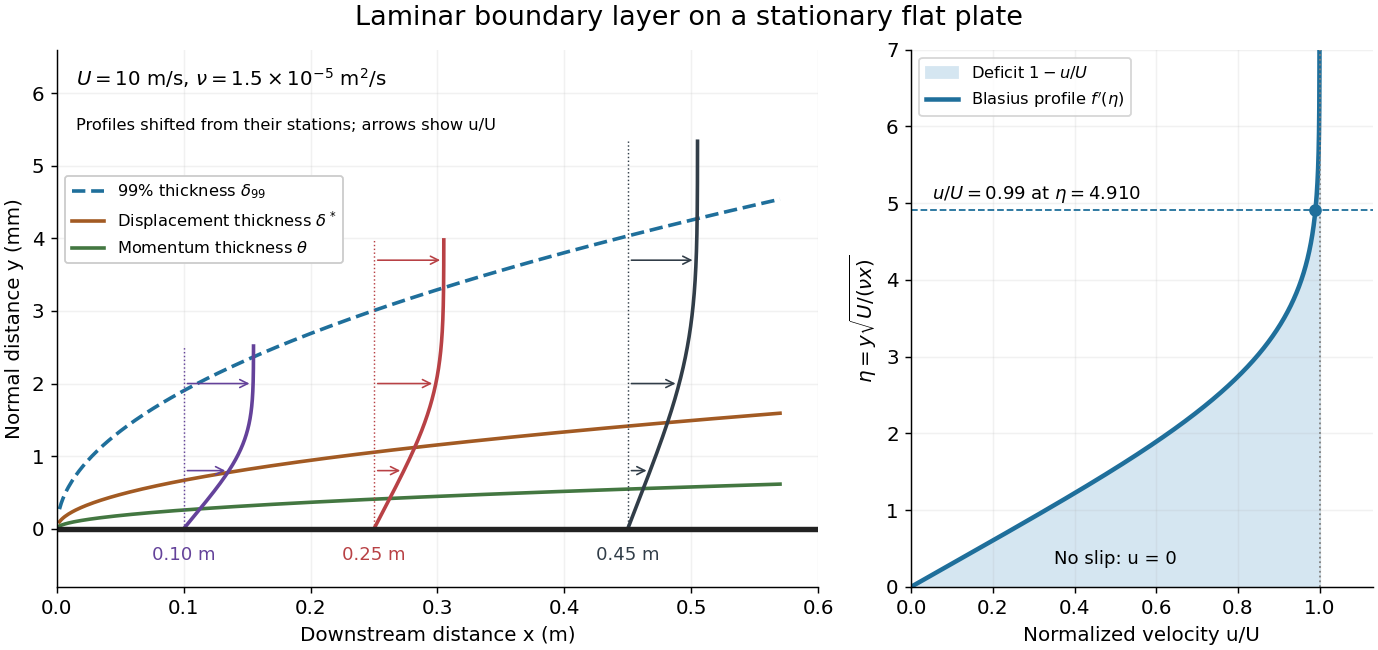
For example, choose $U=10\mathrm{m}{\mathrm{s}}^{-1}$ and $\nu =1.5\times 10^{-5}{\mathrm{m}}^2{\mathrm{s}}^{-1}$. At $x=0.30\mathrm{m}$, the local Reynolds number is ${\mathrm{Re}}_x=Ux/\nu =2.0\times 10^5$ and the boundary layer thickness is about $3.29\mathrm{mm}$. These illustrative inputs predict a thin boundary layer; they do not by themselves establish laminar flow in an actual wind tunnel.

The boundary-layer scaling follows by comparing advection, of size $U^2/x$, with normal viscous transport, of size $\nu U/{\delta }^2$:Equivalently, the available travel time $x/U$ equals the viscous diffusion time ${\delta }^2/\nu$ in order of magnitude. Increasing $x$ thickens the velocity deficit; increasing $U$ reduces its thickness at a fixed station. This boundary-layer scaling requires ${\mathrm{Re}}_x\gg 1$. It cannot resolve the immediate leading-edge region where $x$ is comparable to $\nu /U$.^[ref]

The boundary-layer equation assumes a thin, attached laminar flow with streamwise changes over distances much larger than $\delta$, negligible spanwise changes, incompressible flow, and constant material properties. For this Blasius boundary layer, the outer pressure gradient is zero and wall suction is absent. Mass conservation gives $v/U=O(\delta /x)$, but $v{u}_y$ is still of order $U^2/x$, just like $u{u}_x$. Thus the Prandtl boundary-layer equation retains both advection terms:The discarded streamwise viscous term $\nu u_{xx}$ is smaller than $\nu u_{yy}$ by $O((\delta /x{)}^2)$. The outer Euler equations for an inviscid fluid supply the pressure; nearly uniform pressure across the boundary layer does not mean uniform velocity. Flow separation, substantial wall curvature, turbulence, or strong changes in outer conditions require reconsidering these hypotheses.

Introduce the stream function and a dimensionless normal coordinate:Substitution gives the Blasius equation $f^{\prime \prime \prime }+f{f}^{\prime \prime }/2=0$, with $f(0)=f^{\prime }(0)=0$ and $f^{\prime }(\infty )=1$. Its numerical boundary value problem gives $f^{\prime \prime }(0)\simeq 0.332057$. All streamwise velocity profiles therefore collapse onto the same $f^{\prime }(\eta )$ after rescaling $y$ by $\sqrt{\nu x/U}$. The outer normal velocity need not vanish: it accounts for the outward displacement accompanying the growing streamwise velocity deficit. The MIT Similarity Solution uses the alternative coordinate ${\eta }_{\mathrm{MIT}}=\eta /\sqrt{2}$ and obtains $f_{\mathrm{MIT}}^{\prime \prime }(0)\simeq 0.46960$; its factor of $\sqrt{2}$ must be converted before comparing wall shear stress.

The historical Motion of fluids with very little viscosity by L. Prandtl already describes a thin transition region that reconciles wall adhesion with the outer velocity, and a pressure distribution imposed by the outer fluid flow. Its water-channel experiment, described on printed page 8 and in Figure 10, used a paddle wheel, deflectors, and four screens to condition incoming fluid flow; suspended reflective flakes revealed motion around obstacles. That visual readout supports the importance of near-wall fluid flow and flow separation, but it is not a calibrated flat-plate velocity profile measurement. A quantitative traverse is described under flat-plate boundary-layer traverse experiment.

Electric polarization is electric dipole moment per unit volume. It produces bound volume and surface chargeAcross an interface, the net bound sheet charge is $({\mathbf{P}}_1-{\mathbf{P}}_2)\cdot \mathbf{n}$, where $\mathbf{n}$ points from medium one to medium two.

A string worldsheet $\Sigma$ is the two-dimensional surface swept out by a string in spacetime. Local coordinates are commonly denoted ${\sigma }^{\alpha }=(\tau ,\sigma )$.

Keeping the ordinary reparameterization bc ghost system, four embedding bosons require 44 additional real chiral fermions in each chirality to cancel the worldsheet Weyl anomaly. These are internal matter fields, not an assumed locally supersymmetric RNS construction. Their bilinear currents generate the chiral $\mathfrak{so}(44)$ current algebra, with $\left(\genfrac{}{}{0ex}{}{44}{2}\right)=946$ currents. A full closed fermionic model also requires consistent spin-structure and modular projections; the central-charge count alone does not determine these choices.

Because $X|-⟩=-|-⟩$, a Boolean oracle with answer qubit $|-⟩$ acts as

A polar covalent bond shares electrons unequally, as in hydrogen chloride.

The word “polar” qualifies the sharing within a covalent bond; it does not require complete transfer of an electron or an isolated cation–anion pair. In $A^{\delta +}-B^{\delta -}$, the signs identify the relatively electron-poor and electron-rich ends, while $\delta$ leaves the amount unspecified. A neutral Lewis structure can give both chemical atoms zero formal charge and still correspond to a polar covalent bond: equal division of the bond pair is a formal allocation, whereas bond polarization concerns the actual electron density.

Local and molecular descriptions answer different questions. Calling one chemical bond a polar covalent bond does not establish that the whole molecule is a polar molecule. Combine the bond dipoles with the molecular geometry, then check for molecular dipole cancellation. This lets a short electronegativity comparison explain a local tendency without confusing it with the observable electric dipole moment of the whole molecule.

Opposite forces separated along the unit direction $\mathbf{e}$, with fixed force times separation $D$, have this distributional body force limit. Its net force is zero. A symmetric seismic moment tensor is a sum of such dipoles along its principal directions.

Tight binding approximates a quantum system using orbitals localized near sites and Hamiltonian matrix elements describing their energies and hopping. In a one-dimensional chain with one orbital per cell and nearest-neighbor hopping,A Bloch state gives the dispersion $E(k)={ϵ}_0-2t\cos (ka)$ and bandwidth $4|t|$.

The finite bandwidth makes explicit how overlap between localized states produces delocalized bands. More orbitals, longer-range hopping, spin and magnetic phases give richer matrices. A localized-orbital basis is an approximation to the physical problem, and its parameters must be obtained from a microscopic calculation or fit. The hopping amplitude is a matrix element, not a probability of a completed stochastic hop.

Electronic band structure is the collection of allowed electron energy bands and gaps in a periodic medium, usually represented as energy versus crystal momentum. An energy band is one branch of that structure.

A quantum particle in a one-dimensional lattice experiences a periodic potential. Bloch states organize its spectrum into bands and gaps; the Kronig-Penney model realizes this behavior with an idealized array of barriers or narrow delta barriers.

For $D\ge 4$, the static spherical vacuum metric $d{s}^2=-fd{t}^2+f^{-1}d{r}^2+r^{2}d{\Omega }_{D-2}^2$ has an event horizon at $r_h={\mu }^{1/(D-3)}$. With time normalized at infinity its ADM mass is $M=(D-2){\Omega }_{D-2}\mu /(16\pi G_D)$, where ${\Omega }_{D-2}$ is the unit-sphere area. For $D=5$ and $\mu =2m$, $r_h=\sqrt{2m}$ and $M=3\pi m/(4G_5)$. The spherical orbits are three-spheres, even though the radial-time Penrose diagram has the same causal pattern as its four-dimensional counterpart.