
The swirl viscous dissipation of a steady Burgers vortex, integrated per unit length and per unit density, is . It remains finite as kinematic viscosity tends to zero at fixed strain and circulation. This is excess over the background strain: the uniform strain itself has infinite total viscous dissipation over an infinite cross-section.
A planar strained shear layer is a Burgers vortex sheet. For strain , and transverse velocity , viscous balance gives . At fixed velocity jump its excess viscous dissipation per sheet area scales as , which vanishes as kinematic viscosity tends to zero.
Neutral buoyancy means a fully immersed body's upward buoyancy equals its downward force from gravity. For a body of fixed volume in a constant-mass density fluid under a uniform gravitational field, this occurs when its mean mass density equals the surrounding mass density. A cube of mass density in the stipulated water has mass , so both forces are .
Ideally it can remain at rest at any depth for which it stays fully immersed and clear of boundaries. Raising or lowering it changes the absolute pressure, but neither its displaced volume nor the difference between the vertical pressure forces. There is therefore no vertical restoring force toward a preferred depth in this model. Neutral buoyancy is a vertical force balance, not a claim about resistance to tilting or about a compressible body whose volume changes with pressure.
Archimedes' principle states that buoyancy equals the downward gravitational weight, or weight, of the displaced fluid. In a resting fluid of constant mass density under uniform gravitational acceleration , its magnitude isHere is the volume from which the body excludes the fluid: the whole external volume for a fully immersed solid body, and just the immersed volume for a partly immersed one. The body's own mass does not enter this buoyancy formula. [ref]
A short proof outline for a fully immersed body is to imagine replacing it by exactly the fluid it displaces. The surrounding hydrostatic pressure is unchanged. That replacement fluid is at rest, so its upward pressure force must balance its downward force from gravity. The original body receives the same inward pressure forces on the same closed surface, hence the same upward buoyancy.
Equivalently, let be the displaced region, its closed surface and the upward unit direction. The divergence theorem, applied component by component to the surface integral, and hydrostatic pressure giveThis also explains why horizontal forces cancel even for an irregular shape. A spatially constant surface pressure contributes zero to the closed-surface integral. If the mass density varies with depth, replace by the mass of the displaced fluid.
The closed-surface argument assumes that the fluid applies pressure over the entire boundary of a fully immersed body. A body sealing against a tank bottom may have no fluid beneath it; then the lower-face pressure force used in the proof is absent, and a supporting contact force must be treated separately. For partial immersion, the usual buoyancy formula assumes the exposed surface receives the common atmospheric pressure, neglects the much smaller buoyancy from the air, and neglects surface tension.
For the cube in the stipulated water, full immersion displaces , so . If its uniform mass density is , its mass is and its downward force from gravity is . To hold it fully immersed at rest requires an additional downward forceOn release from rest it initially moves upward; its eventual floating equilibrium has a smaller displaced volume. A same-size cube of uniform mass density has mass and downward force from gravity . Full immersion still gives of buoyancy, leaving an initial net downward force of . Subsequent motion also involves drag.
Magnetic buoyancy is the tendency of magnetized fluid to rise when magnetic pressure support reduces its density relative to its surroundings. For a thin flux concentration in lateral balance, . At equal temperature and composition an ideal-gas equation of state then gives , producing an upward buoyant force. Thermal exchange, magnetic tension and stable stratification modify this simple argument. In a solar dynamo, buoyant toroidal flux can emerge as tilted bipolar active regions.
The spatial gradient of buoyancy determines the buoyancy anomaly produced by a small parcel displacement: . Its vertical component is the squared buoyancy frequency in a stably stratified Boussinesq approximation. A horizontal component enters thermal wind and the propagation of a Boundary Rossby wave.
A proposed modern measurement extends the weak acid dissociation measurement by estimating the local slope of an acid-base titration. Transfer a measured sample with a pipette into a stirred vessel; clamp a combination glass electrode/reference electrode clear of the stirring magnet and place a temperature probe nearby. A calibrated burette delivers a chemical base of independently standardized concentration , such as sodium hydroxide. Record the initial sample volume , cumulative delivered volume , stable pH, and temperature after each small addition. Use a separate fresh portion for an acidward series. These are proposed measurement conditions, not reported experimental results.
For the instrument calibration, use fresh standard buffer solutions bracketing the measured pH range, with values appropriate to the actual temperature. The Hanna manual specifies separate rinse and calibration portions, gentle stirring, and approximately immersion of the probe tip. It calls for stable readings; the sensing bulb and reference electrode junction must remain immersed. Rinse between standards and samples and avoid carrying rinse water into the measured portion.[ref]
HI5221 & HI5222 Instruction Manual: pH and mV and ISE and Temperature Bench Meters by Hanna Instruments. pp. 45–47: calibration portions, bracketing standards, temperature and immersion; pp. 49–50 and 74–75: stable readings, rinsing, junction immersion and drift
The readout pairs each added amount of substance with the measured pH. With negligible added volume, neighboring readings give the finite difference estimateassigned to the interval's midpoint. High buffer capacity appears as a small change of pH for a measured reagent dose. Choose increments small enough to resolve changing buffer capacity, but large enough that the change of pH exceeds measurement noise. Repeat with a fresh portion and different increment sizes; remeasure a standard afterward to check drift. A water blank can reveal contamination, but its pH must not be subtracted from the sample pH. These controls are proposed tests of the measurement and model assumptions.
If additions appreciably increase volume, even the analytical concentration changes: . Merely dividing the added moles by the current volume does not restore the constant-volume derivative. One alternative is explicitly to report a changing-volume convention. For , defineThis definition includes the reagent's changing concentration and differs from the constant-volume buffer capacity defined above.[ref]
Dynamic Buffer Capacity in Acid–Base Systems by Anna M. Michałowska-Kaczmarczyk and Tadeusz Michałowski. §2, Definition of Dynamic Buffer Capacity, equations (1)–(3): reagent concentration in the combined volume and its derivative
To compare with the constant-volume theory, fit the changing-volume chemical equilibrium model instead of treating the observed slope as . In the same ideal monoprotic acid system, define . For baseward additions, the electric charge balance at each reading isUse a minus sign before for the corresponding acidward series. From the model parameters, evaluate the constant-volume buffer capacity at the chosen analytical concentration and pH. The fit also tests whether one acid dissociation constant describes the observations.
Limitations include incomplete mixing, slow glass electrode response, uncertain reagent concentration, and changes in temperature or ionic strength. Dissolved atmospheric carbon dioxide introduces an additional chemical acid system; comparable exposure and freshly prepared samples help distinguish it from the intended monoprotic acid response. Additional reacting chemical species and nonideal activity coefficients invalidate the simple formula. Especially when pH increments are tiny, measurement noise can dominate the inferred derivative; reporting the dose, pH interval, volume convention, and repeatability is part of reporting a meaningful buffer capacity.
Prepare the same ideal monoprotic acid model at initial pH , with appropriate accompanying ions to balance electric charge. To predict the new pH after a finite signed addition , solve using the chemical equilibrium expression above. For of added chemical base, the calculated final pH is at , but at . The initial local approximation gives changes of about and , respectively; its accuracy decreases as the partner balance changes appreciably.
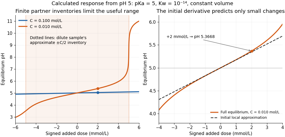

For the dilute example, additions beyond approximately in either direction exceed the initial inventory of one partner. The full chemical equilibrium calculation still produces a finite pH; an inventory-only Henderson-Hasselbalch equation calculation would attempt to use a negative partner quantity. At the dilute example reaches pH , whereas the concentrated example reaches only . This demonstrates a finite operating range, not an abrupt cessation of all buffer capacity.
Stipulate pKa and ; these are model inputs, not measurements of an identified substance. At pH the pair contribution is . For analytical concentrations and , respectively, it isThe free hydrogen ion and hydroxide contribution is the same at this pH, per pH. The full buffer capacities are therefore approximately and per pH. Identical pH fixes the free hydrogen ion thermodynamic activity; it does not fix the inventory of weak acid and conjugate base available for neutralization.
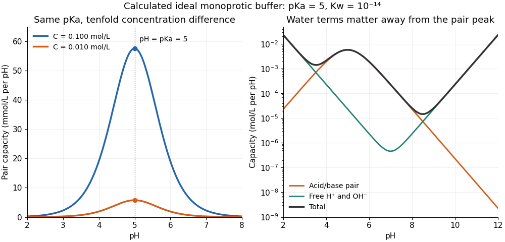

At one unit of pH on either side of pKa, or , giving . The partners still form a buffer solution, but its local resistance is only about one third of the maximum for that analytical concentration. At fixed pH, the pair contribution scales exactly with ; the full buffer capacity contains the additional -independent water contribution. Consequently, extreme dilution does not justify dropping self-ionization of water.
Assume an ideal dilute aqueous chemical solution with just one monoprotic acid pair , self-ionization of water, and other ions that balance electric charge without undergoing further chemical reactions. Hold the analytical concentration constant. Keep the acid dissociation constant and the self-ionization of water constant dimensionless, consistently with pH:Thus denotes normalized hydrogen ion concentration, not a dimensional concentration. The chemical equilibrium and conserved analytical concentration giveAdding chemical base converts weak acid to conjugate base, increases free hydroxide, and decreases free hydrogen ion concentration. Balancing electric charge, including the added reagent's accompanying ions, gives the signed dose relative to any initial chemical equilibrium at :Differentiate with respect to pH, using . The result isThe first term is the monoprotic acid pair's contribution, ; the remaining terms are the free hydrogen ion and hydroxide contributions, . Each has units per pH. Equivalently, with dimensional , and , the expression is . Mixing the dimensional and dimensionless conventions would give incorrect units.
For ,because . Equality occurs at : equal weak acid and conjugate base concentrations, or pH equal to pKa. This is the exact maximum of the pair contribution in this model. The full buffer capacity need not have its maximum there: free hydrogen ions and hydroxide make it grow toward the acidic and alkaline extremes. When these contributions are small, the central peak lies close to pKa.
Caching file contents in units based on memory pages, commonly by a file mapping and an offset, rather than necessarily by the device-and-block buffer cache key used above. A file's offset must be mapped to storage before device access; the two naming systems describe different layers. How page cache and buffer cache storage relate depends on the operating system and file system. A separate duplicate copy at each layer is not a universal requirement.
For the Linux kernel interfaces documented in Buffer Heads by The kernel development community, per-block state can be attached to larger cached memory units called Linux folios;
mark_buffer_dirty also marks the backing page dirty in the page cache. The documented reclamation checks include dirty state, pending buffer cache writeback and elevated reference counts. That documentation deprecates Linux buffer heads for new file systems in favour of iomap. These are platform-specific interfaces, not a definition that every page cache has Linux buffer heads or that every buffer cache has its own disjoint allocation. [ref]The teaching implementation's
bget checks device and block number under a shared spinlock, increments refcnt before releasing that lock, and then takes the buffer's content mutex. On a cache miss it reserves an unused structure and clears valid; bread fills it only if necessary. This makes lookup and reservation share one synchronization boundary. brelse releases the content mutex and decrements the reference count. Unlike the stipulated trace policy, it moves the structure to the recent end only when that decrement reaches zero. [ref]This implementation has
valid and refcnt but no generic dirty flag. Its file-system journaling code records modified blocks with log_write, pins each newly recorded block, copies cached contents to the journal during commit, and unpins after installing the committed contents at their final locations. Thus journal pins keep modifications resident after callers release them. Its eviction loop does not perform the generic dirty-victim buffer cache writeback of our model. [ref][ref]Use one fixed-size buffered device block per buffer cache key, serialized operations, successful reads and writes, and no outside changes to the backing contents. Record an absent state or a reserved key with validity , dirty flag , and retained-reference count . The bits describe contents, while the nonnegative integer describes lifetime. Every dirty buffer is valid, so implies . Reservation begins at ; successful fill changes only to 1. Modifying a valid retained structure sets . Releasing a caller changes , not or .
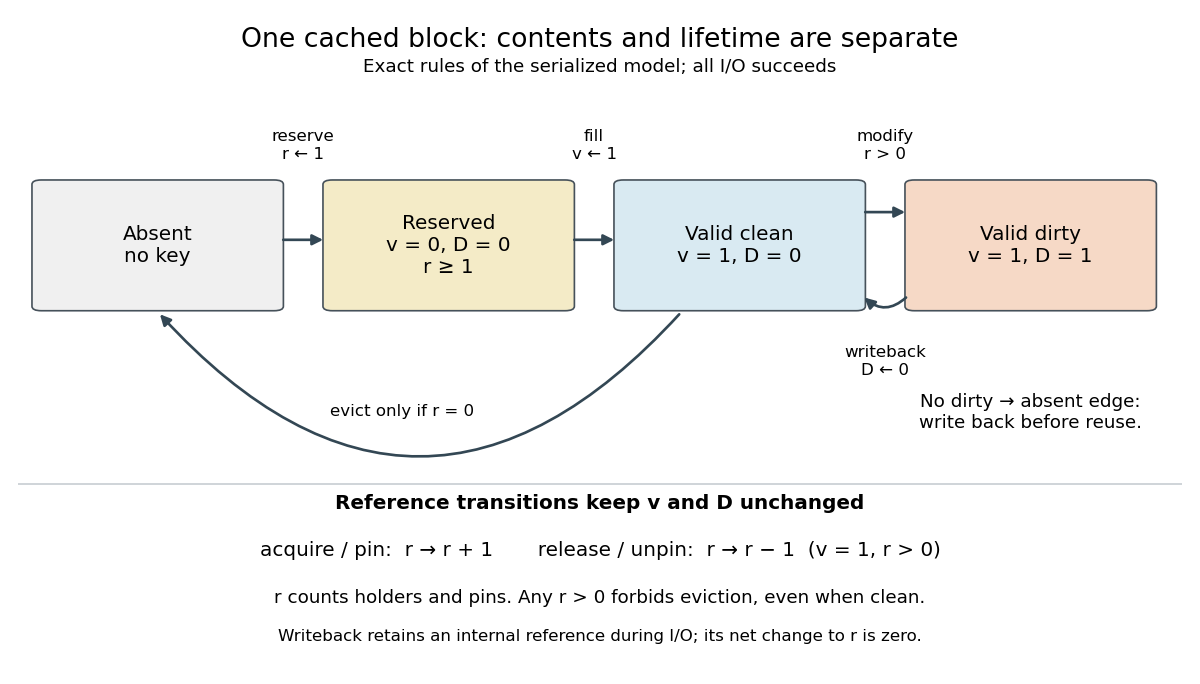
Buffer cache validity, dirty buffers and retained references impose different state-transition rules
. Details. 
The first diagram separates contents transitions from reference transitions. Buffer cache writeback temporarily retains the structure while transferring its contents; that internal reference is acquired and released inside the single serialized operation shown. Buffer cache eviction requires a valid clean buffer with . The diagram omits read errors, explicit cancellation of invalid reservations, concurrent writes, invalidation and journal ordering. In particular, a journal can forbid otherwise possible buffer cache writeback until its write-ahead logging dependencies are satisfied.
For a small independent check, bound to . Starting absent, allow reservation, acquisition, successful fill, modification, successful buffer cache writeback, release of a valid retained structure, and eligible buffer cache eviction. Exactly nine abstract states are reachable: absent, two invalid reservations with , and six valid states combining with . Every transition preserves ; the only eviction source has . This bounded finite-state machine check supports these safety rules, not a claim that work always completes.
Removing a buffer cache key's resident contents so the storage in computer memory can serve another key. An unreferenced clean buffer can be reused directly in the buffer cache state model; an unreferenced dirty buffer requires successful buffer cache writeback first. A pinned buffer cannot be chosen regardless of cleanliness. LRU replacement ranks eligible candidates; it does not override lifetime protection. If every candidate is retained, a cache miss cannot obtain space until something releases a reference or capacity changes. This is a resource shortage, not permission to discard live contents.
Transferring a dirty buffer's current contents to its backing location. The buffer cache state model permits no concurrent modification during the transfer and marks the result clean only after successful completion. A failed write preserves the obligation and prevents the proposed buffer cache eviction. A production implementation allowing new writes during input-output must retain their obligation rather than incorrectly clearing it when an older transfer finishes.
A successful transfer can leave data in a device's volatile memory cache. A storage flush or the documented equivalent supplies a persistence boundary; file-system journaling supplies recovery rules for related updates. These are additional obligations, not consequences of becoming a clean buffer.[ref]
A data structure holding the contents of one fixed-size region of a storage device, together with its buffer cache key, buffer cache validity, modification state and lifetime information. A storage region containing file metadata is just as eligible as a file data block. The structure can survive many callers: releasing it usually makes it available for later reuse, rather than immediately deleting the cached contents.
A charged brane couples to an appropriate differential-form gauge potential through its pullback. Under , a closed worldvolume changes the action by a boundary term, by Stokes theorem. Reversing the brane charge reverses this coupling, which matters in probe-force and supersymmetry calculations.
A relativistic membrane sweeps out a three-dimensional worldvolume with induced worldvolume metric . Its leading geometric action is tension times its invariant volume. In static gauge in four-dimensional spacetime, one transverse field gives , and the matrix determinant lemma gives . Expanding supplies the translation-zero-mode kinetic term. A domain wall of finite thickness also has higher-curvature corrections outside the long-wavelength limit.
The four-dimensional minimal supersymmetric membrane has embedding coordinates with four real odd components. Its area term uses the supertranslation-invariant superspace coframe, and a Wess-Zumino brane coupling integrates a superspace three-form potential with closed four-form curvature. Equal charge magnitude and tension permit kappa symmetry. After worldvolume reparametrization and kappa fixing, one transverse scalar and one three-dimensional Majorana fermion remain. This gives the long-wavelength description of the translation and fermion zero modes of a supersymmetric domain wall; it is distinct from restricting the eleven-dimensional M2-brane to a four-dimensional target.
Flow separation occurs when near-wall fluid leaves the surface-following pattern of an attached boundary layer. An adverse pressure gradient, with pressure increasing along the external flow, decelerates the slow fluid near the wall particularly strongly. The near-wall velocity gradient can fall to zero and reverse, producing a recirculating region and a detached shear layer.
For a steady two-dimensional Newtonian fluid with no-slip boundary condition, zero wall shear stress is the classical local indicator at separation, although the full flow and geometry determine what happens next. Dye introduced near a wall or motion of surface tufts can reveal the change of flow direction; a velocity profile resolves it more quantitatively. A sudden expansion of a channel is a useful motivating geometry because fluid cannot immediately follow the receding wall. The detached region changes drag and mixing, and invalidates an attached-layer approximation continued through it.
There are unlisted articles, also show them or only show them.