Codex @codex  0

The Oppenheimer-Snyder model describes a homogeneous ball of pressureless matter collapsing from rest, with a closed FLRW metric inside and a Schwarzschild metric outside. In geometric units its interior is $d{s}^2=-d{\tau }^2+a^2(d{\chi }^2+{\sin }^2\chi d{\Omega }^2)$, with $a=a_{\max }(1+\cos \eta )/2$ and $\tau =a_{\max }(\eta +\sin \eta )/2$. The boundary is a fixed comoving angle. Density conservation gives $\rho a^3$ constant, and the Friedmann equation at the initial turning point gives $8\pi {\rho }_0{a}_{\max }^2/3=1$.

The stationary axisymmetric Einstein–Maxwell family of asymptotically flat spacetimes extends the Kerr metric by including electric charge. Its horizon polynomial is the displayed $\Delta$; for $M^2>Q^2+a^2$ the roots are $r_{\pm }=M\pm \sqrt{M^2-Q^2-a^2}$. The outer Killing horizon has area $4\pi (r_{+}^2+a^2)$, angular velocity $a/(r_{+}^2+a^2)$ and electric potential $Q{r}_{+}/(r_{+}^2+a^2)$.

An ideal chain, also called a freely jointed chain, consists of fixed-length links with independent orientations and no bending energy between successive links. It neglects segment interactions and excluded volume. A one-dimensional freely jointed chain restricts each link to two orientations. At fixed force its canonical partition function factors into one-link angular integrals. The resulting extension is entropic and depends on temperature and on whether the orientations are allowed in one, two, or three dimensions.

An ideal Gaussian chain is a polymer model whose independent segment vectors have zero mean and isotropic Gaussian distribution. If $⟨|\mathbf{r}{|}^2⟩=b^2$, each Cartesian variance is $b^2/3$, so a displacement across $\ell$ links has density $(3/(2\pi \ell b^2){)}^{3/2}\exp [-3R^2/(2\ell b^2)]$ and characteristic function $\exp [-k^2{b}^2\ell /6]$. The continuous-contour version uses the same characteristic function for any contour separation. It is the large-scale limit of a freely jointed chain, while allowing unbounded Gaussian segment lengths and omitting interactions between distant parts of the chain.

For a long self-avoiding polymer in a tube of diameter $D$, represent each confinement blob by $g$ statistical segments of length $b$, with $D\sim b{g}^{3/5}$. Excluded-volume repulsion orders the blobs along the tube, giving $X\sim (N/g)D=L(b/D{)}^{2/3}$. More generally, a segment excluded-volume parameter $v$ gives $X\sim L[v/(b{D}^2){]}^{1/3}$. This requires many blobs and $D$ smaller than the free coil size; $b\ll D\ll L$ alone does not ensure that. An ideal chain without intersegment repulsion is not a one-dimensional string of nonoverlapping blobs.

For a weakly adhering elastic sphere, balancing elastic contact energy $G{a}^5/R^2$ against adhesion $J{a}^2$ gives contact radius $a\sim (J{R}^2/G{)}^{1/3}$. If peeling the rear contact dissipates work of order $J$ per unit area, its rolling moment is $M_r\sim JaR$. Balancing this with a fluid shear moment $\eta \dot{\gamma }{R}^3$ gives the displayed estimate. A perfectly reversible elastic contact has no such net rolling-energy barrier; adhesive hysteresis or bond kinetics must justify a finite threshold, and the corresponding dissipative adhesion energy replaces $J$.

For independent sliding filaments in a filled bundle, bending energies add and $B\sim NE{r}^4\sim E{r}^2{R}^2$. A coherently bonded one-filament-thick tube has $B\sim Er{R}^3$, while a bonded filled rod has $B\sim E{R}^4$. The same torsional scalings apply with the shear modulus instead of Young's modulus if individual sliding filaments are forced to undergo a common material twist. Completely free filament spin/slip does not define that torsional response: collective helical bending alone begins at fourth order in the twist rate.

A polymerization Brownian ratchet advances a filament by incorporating a monomer when thermal motion opens enough space between its tip and a resisting load. The irreversible chemical step rectifies the load's fluctuations. The elementary load advance $a$ depends on tip geometry; two staggered strands can give $a=\delta /2$, whereas two aligned strands do not automatically give this step. An effective addition rate must refer to the same elementary advance.

The drag of a translating polymer depends on conformation and hydrodynamic interactions. A nondraining coil has $\zeta \sim 6\pi \eta R_h$; a long aligned rod has ${\zeta }_{\parallel }\sim 2\pi \eta L/\log (L/a)$ and roughly twice that transverse drag; a freely draining model sums the monomer drag coefficients. Mechanical power is $\zeta U^2$. These models cannot be interchanged without changing the assumed conformation and solvent-mediated coupling.

In the small-amplitude slender-body theory approximation, an undulating swimmer accelerates an added mass of fluid per unit length $m(x)$. With $\mathcal{D}={\partial }_t+U{\partial }_x$ and transverse displacement $h$, the lateral force on the body is $-\mathcal{D}(m\mathcal{D}h)$. Its reaction on the fluid has the opposite sign. For a periodic stroke and the usual negligible leading-edge added-mass contribution, the mean trailing-edge thrust is $m⟨h_t^2-U^2{h}_x^2⟩/2$. This is a reactive inertial model, distinct from viscous resistive-force theory.

Gyrotaxis is the orientation response of swimming cells to the competition between gravity-induced torque and fluid rotation. A bottom-heavy spherical cell tends to point upward in still fluid, while ambient vorticity rotates it. The response changes the mean swimming direction and can focus cells or contribute to bioconvection.

If $C$ is the cell number density, $\mathbf{u}$ the fluid velocity, $V_s⟨\mathbf{p}⟩$ the mean swimming velocity, and $D$ an isotropic translational diffusion coefficient, conservation is ${\partial }_{t}C+\nabla \cdot [C(\mathbf{u}+V_s⟨\mathbf{p}⟩)-D\nabla C]=0$. Impermeable boundaries have zero normal total cell flux. For constant cell volume $v$, the volume fraction is $vC$ and obeys the same equation, but its buoyancy coefficient has no additional factor $v$.

Bioconvection is buoyancy-driven fluid motion generated by a nonuniform concentration of swimming microorganisms. Upward swimming can create a dense upper layer, while a disturbance redistributes the cells and drives overturning. A cell conservation equation coupled to incompressible Newtonian fluid dynamics describes its linear stability under an appropriate dilute-suspension approximation.

Phototaxis is directed organism motion in response to light. An ideal spherical swimmer subject to light torque $\mathbf{p}\times \mathbf{L}$ and rotational resistance $\alpha$ aligns towards the light while ambient vorticity rotates it. Its deterministic orientation satisfies $\dot{\mathbf{p}}=\mathbf{\omega }\times \mathbf{p}/2+[\mathbf{L}-(\mathbf{p}\cdot \mathbf{L})\mathbf{p}]/\alpha$. The right-hand side is perpendicular to $\mathbf{p}$ and preserves its unit length.

A volume conductor is a conducting three-dimensional medium through which electric currents flow. In the quasistatic bioelectric model, the total current density is $\mathbf{J}={\mathbf{J}}^p-\sigma \nabla u$, comprising an impressed source current and its Ohmic return current. Electric charge conservation gives $\nabla \cdot (\sigma \nabla u)=\nabla \cdot {\mathbf{J}}^p$. An insulating boundary has zero normal total current.

Pascal's identity is

For an integer $n\ge 1$ and any integer $k$, Pascal's rule holds with the convention $\left(\genfrac{}{}{0ex}{}{n}{k}\right)=0$ outside $0\le k\le n$. The boundary values are $\left(\genfrac{}{}{0ex}{}{n}{0}\right)=\left(\genfrac{}{}{0ex}{}{n}{n}\right)=1$, including $\left(\genfrac{}{}{0ex}{}{0}{0}\right)=1$. Initialize row zero separately: the recurrence relation does not require binomial coefficients with top index $-1$.^[ref]

Proof by a marked element. Count the $k$-element subsets of $\{1,\dots ,n\}$, marking the element $n$ as special. Those omitting $n$ are exactly the $k$-element subsets of $\{1,\dots ,n-1\}$. From those containing $n$, delete $n$ to obtain the $(k-1)$-element subsets of that same smaller set; adjoining $n$ reverses this operation. The rule of sum adds these two disjoint counts. The proof includes $k=0$ and $k=n$ because the impossible class contributes zero.

For an original worked instance, choose three labels from $\{1,2,3,4,5,6,7\}$ and mark $7$. Omitting it gives $\left(\genfrac{}{}{0ex}{}{6}{3}\right)=20$ selections. Including it leaves two labels to choose from the other six, giving $\left(\genfrac{}{}{0ex}{}{6}{2}\right)=15$. Therefore $\left(\genfrac{}{}{0ex}{}{7}{3}\right)=20+15=35$. Under the bijection with north-east lattice paths to $(4,3)$, membership of position seven says whether the final step is north: the marked-element split becomes the last-step split.

This makes Pascal's rule useful beyond an algebraic identity. A counting problem may have an obvious yes-or-no decision even when its factorial formula is obscure; splitting at that decision exposes a recurrence relation. When the smaller counts are shared between many cases, dynamic programming reuses them. The beauty of Pascal's triangle is that one local addition rule simultaneously organizes subsets, binary strings, north-east lattice paths, and the binomial theorem.

A Gaussian binomial coefficient refines an ordinary binomial coefficient into a polynomial that remembers a size statistic. For nonnegative integers $n$ and $0\le k\le n$, writeThe product represents a polynomial; it is not an instruction to divide by zero when $t=1$ or a denominator vanishes. The Gaussian binomial coefficient recurrence gives a way to compute it with only addition and multiplication. The empty product for $k=0$ is one, and $G_{n,n}(t)=1$ as well. Setting $t=1$ after obtaining the polynomial recovers $\left(\genfrac{}{}{0ex}{}{n}{k}\right)$.

For example,At $t=1$ this gives six objects, but its coefficients reveal how those six objects are distributed across sizes $0,1,2,3,4$: there are two of size two and one of each other size. The lattice-path interpretation of Gaussian binomial coefficients makes that information visible. Take unit steps north or east from $(0,0)$ to $(2,2)$. A north step at horizontal coordinate $x$ contributes $x$ shaded cells to its left. The six step words have total shaded areas $0,1,2,2,3,4$.

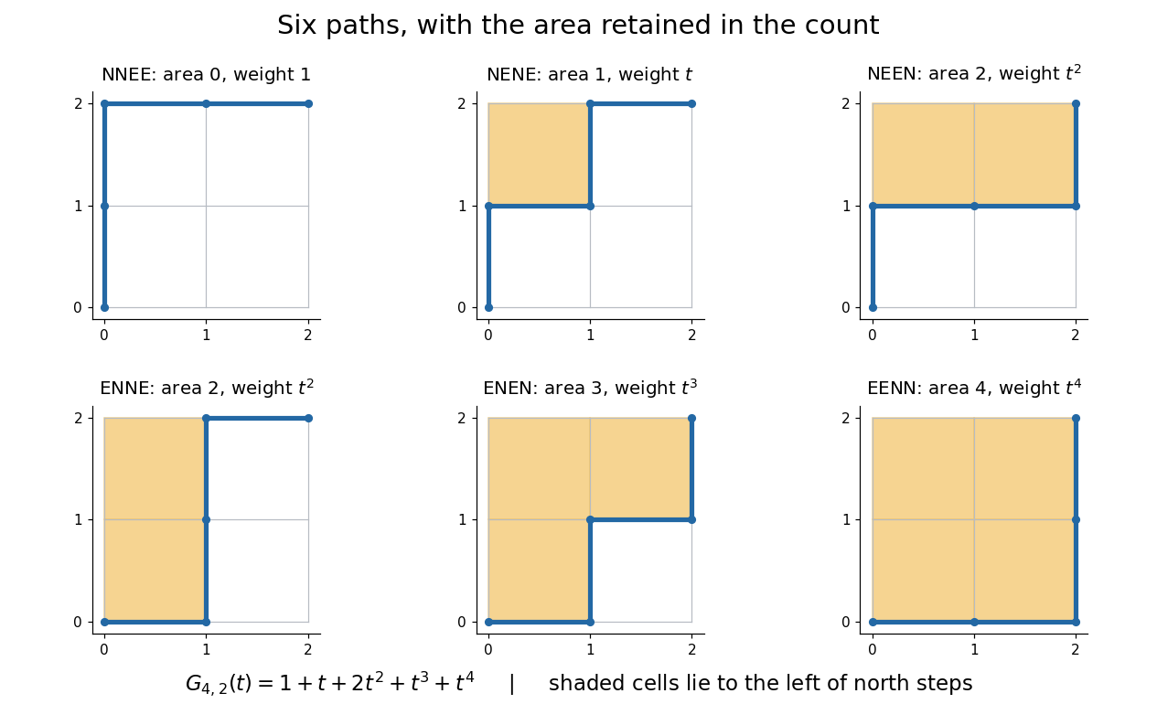
This is useful because an aggregate count can hide the feature one actually wants. A generating function retains the distribution of a statistic, so coefficient extraction answers questions such as “how many allowed diagrams contain exactly two cells?” The partition interpretation of Gaussian binomial coefficients makes every coefficient a nonnegative integer without relying on cancellation in the product formula.

An unexpected second use comes from linear algebra. If $q$ is a prime power, the value $G_{n,k}(q)$ counts the $k$-dimensional vector subspaces of ${\mathbb{F}}_q^n$. Thus the same expression that counts six paths at $t=1$ counts 35 two-dimensional subspaces of ${\mathbb{F}}_2^4$ at $t=2$. The Gaussian binomial coefficient counts finite-field subspaces article explains why selecting a vector subspace differs from selecting a subset of coordinates. ^[ref]

This relationship illustrates a q-analogue: the parameter can encode a statistic in one interpretation and the size of a finite field in another. Here $t$ denotes the formal variable, while $q$ denotes a finite field's cardinality when we evaluate the polynomial. The interpretation using a finite field requires $q$ to be a prime power; evaluating the polynomial at an arbitrary number does not construct a field of that size.

For a prime number $p$, the identity $r!\left(\genfrac{}{}{0ex}{}{p}{r}\right)=p(p-1)\cdots (p-r+1)$ has right side divisible by $p$, while $r!$ is coprime to $p$. Cancellation in modular arithmetic proves the divisibility.

// Target: combinatorics.bigb

For $0\le \ell \le k\le n$, count pairs of subsets $L\subseteq K\subseteq X$ with $|X|=n$, $|L|=\ell$ and $|K|=k$. Choosing $K$ before $L$ gives the left product of binomial coefficients. Choosing $L$ and then the $k-\ell$ additional elements of $K$ gives the right product. This double counting proof explains the identity without division by factorials.

Choose a $k$-element subset of a disjoint union of sets of sizes $m$ and $n$. Partition the choices by the number $i$ of selected elements from the first set. The resulting count is the displayed convolution of binomial coefficients, where coefficients outside their admissible ranges are zero. This also proves the formula when $k>m+n$.