Past exam of the mathematics course of the University of Cambridge 2006 iii Paper 31 4 ii Solution by  Codex 0 Created 2026-10-03 Updated 2026-10-14
Let be the Cameron-Martin space of Wiener measure on : its elements start at zero, are absolutely continuous, and have square-integrable derivatives. For , let solve the controlled ordinary differential equationThe Stroock-Varadhan support theorem in the uniform topology isOne may equivalently take piecewise linear or smooth controls starting at zero. The skeleton uses the displayed vector fields, as appropriate for the Stratonovich equation.
Choose and work in the complete separable space of anchored geometric p-rough paths, with its rough path metric . The enhanced Brownian motion is a random element of this space. Its support of a measure isWe explain this Brownian support step using the permitted results about the enhancement. The almost-sure polygonal convergence proved in Question 3 gives the inclusion of its support in . Indeed, polygonal controls belong to , and the enhancement belongs to their closed signature closure almost surely. Hölder rough-path convergence at an exponent greater than implies -variation convergence: for the level- differences, sum the bound proportional to over a partition. Since , these sums are uniformly bounded and tend to zero with the Hölder distance.
For the reverse inclusion, use Brownian rough path small-ball positivity, namely for every , and Cameron-Martin quasi-invariance of enhanced Brownian motion. These are the Brownian input results used without proof here. For , the rough path translation is continuous and sends to . The law of is equivalent to that of . Given an open neighborhood of , continuity supplies an identity neighborhood mapped into . Small-ball positivity gives positive probability that ; equivalence of the two laws gives . Hence belongs to the Brownian support for every . Closedness of support proves the equality with .
Let be the state-path solution map of the rough differential equation driven by these vector fields, with the fixed initial value . The assumed identification of the Stratonovich solution says . Boundedness of the fields and all their derivatives ensures global existence and the regularity needed by the universal limit theorem. That theorem makes continuous from the rough-path space into the uniform state-path space. For a control signature, consistency with ordinary equations gives .
We use the elementary support under a continuous map identityTo prove it, a neighborhood of with has an open inverse image containing , and therefore positive measure. This puts , and its closure, in the image support. Conversely, the image closure is closed and has full image measure, since the original support has full measure. The minimal closed full-measure characterization from Question 4(i) gives the other inclusion.
Apply this identity to and the Brownian rough-path law. We obtainContinuity and the definition of imply . The reverse inclusion after taking closures follows from . Therefore the last displayed support is exactly the uniform closure of the skeleton paths, proving the theorem.
Finally, piecewise constant and smooth approximations of converge in , hence in on a finite interval. Their controls converge in total variation, their signatures converge in the rough-path metric, and the universal limit theorem gives uniform convergence of the corresponding skeleton solutions. This proves the stated equivalence of the control classes.
Past exam of the mathematics course of the University of Cambridge 2006 iii Paper 31 4 i Solution by Codex 0 Created 2026-10-03 Updated 2026-10-14
Codex 0 Created 2026-10-03 Updated 2026-10-14For a Borel probability measure on a Polish space , its support of a measure isEquivalently, for a compatible metric, every open ball about has positive measure. The complement is open: any zero-measure open neighborhood of a point is a zero-measure neighborhood of all its points. Hence the support is closed.
A Polish space has a countable base. Its support complement is therefore a countable union of zero-measure basic open sets, so . If is any closed full-measure set, a point outside has the zero-measure open neighborhood and is outside the support. Thus the support is also the smallest closed set of full measure. Countability is what justifies the full-measure assertion; an arbitrary uncountable union of null sets would not suffice.
Past exam of the mathematics course of the University of Cambridge 2006 iii Paper 31 3 ii Solution by Codex 0 Created 2026-10-03 Updated 2026-10-14
Codex 0 Created 2026-10-03 Updated 2026-10-14Put . These sigma-fields increase, and their union generates the continuous Brownian path. Let be the polygonal enhancement. Its coordinates are determined by its displacement and antisymmetric area ; the symmetric second level is .
The given conditional-expectation identities implyFor the second assertion it is important to use area coordinates rather than asserting that the whole tensor signature is a conditional expectation. Write . The local off-diagonal second integral isConditional on their separate dyadic values, the two independent Brownian components remain independent. Thus the conditional expectation of the product in the last term is . The assumed identity for gives the polygonal entry. The reverse entry follows by integration by parts, since the product of the two component increments also has the product of their conditional means. Taking the antisymmetric part proves the area identity. Diagonal second levels are recovered from the geometric identity, rather than from a conditional-expectation claim about squares.
For each fixed dyadic time , the first-level and area conditional expectations are uniformly integrable martingales in . Their targets are measurable with respect to : Brownian area is a limit of stochastic integral sums determined by the path. The martingale convergence theorem gives convergence to and , respectively. The continuous group coordinate formulas then giveat all dyadic times on a common event of probability one.
For the uniform Hölder estimate, fix and put . The given all-order integrability and the group norm comparison implyUse the conditional-expectation formulas, the conditional Jensen inequality, and . The group norm comparison yieldsFirst take all dyadic pairs, a countable collection, and then extend the inequality to all by continuity. Hence the Brownian rough path martingale Hölder bound isFor any , the Doob Lp maximal inequality givesTherefore
To upgrade convergence from dyadic times to every time simultaneously, apply this bound at one positive exponent . The polygonal enhancements are then equicontinuous in the group metric, with a common finite random constant. For a finite dyadic time net, convergence holds at every net point. The triangle inequality bounds the errors at the remaining times by the two Hölder errors to the nearest net point and the error at that point. First let , and then let the net mesh tend to zero. This proves uniform convergence, and in particular convergence for every on one event of probability one.
There is also convergence in each weaker Hölder rough path metric. Uniform convergence of the group coordinates gives uniform convergence of their levelwise increments through the Chen formulas. If , the uniform bounds bound the level- increment differences by a random constant times , while their unweighted suprema tend to zero. Interpolating these two bounds proves convergence with denominators , for . This establishes the nested polygonal approximation of Brownian rough paths in the topology needed for the support argument.
Past exam of the mathematics course of the University of Cambridge 2006 iii Paper 31 3 i Solution by Codex 0 Created 2026-10-03 Updated 2026-10-14
Codex 0 Created 2026-10-03 Updated 2026-10-14For Brownian motion starting at zero, define its enhanced Brownian motion by the Stratonovich second level:The associated group-valued path is . The Stratonovich chain rule givesConsequently its symmetric second level is and the remaining antisymmetric part is Lévy area. Splitting the integral at proves the Chen identity, so these increments lie in and are the relative increments of .
The group norm for the Carnot-Carathéodory distance is comparable to . The planar construction in Question 2 extends to dimension : prescribe every coordinate-plane area with a closed rectangle, concatenate these central-area loops, and finish with the displacement segment. The converse bound follows from length bounds on displacement and on each area integral. Thus the comparison constants depend only on .
Brownian scaling and stationarity of increments imply that has the distribution of . The permitted moment estimates for Lévy area, together with Gaussian moments of Brownian displacement, therefore give, for every finite ,This also verifies the hypothesis of the metric-valued Kolmogorov continuity theorem. We give the dyadic argument to obtain a simultaneous version explicitly.
Fix and choose so large that . The Markov inequality and a union bound giveThe right-hand side is summable. By the Borel-Cantelli first lemma, almost surely there is a finite random constant bounding every adjacent dyadic increment by , including the finitely many exceptional levels.
Decompose any interval with dyadic endpoints into successive dyadic intervals, with at most two intervals of each size and no size exceeding its length. The metric triangle inequality and the sum of the geometric series givefor all dyadic . The finite-dimensional Carnot group is complete, so the path extends uniquely from dyadic times to a continuous -Hölder path. At each fixed time the original stochastic enhancement and its values at approaching dyadic times converge in probability by the moment estimate. The extension has the same limit almost surely, hence is a modification of the original enhancement.
Past exam of the mathematics course of the University of Cambridge 2006 iii Paper 31 1 ii Solution by Codex 0 Created 2026-10-03 Updated 2026-10-14
Codex 0 Created 2026-10-03 Updated 2026-10-14Let be a weak geometric p-rough path, , with increments indexed by words of length at most . Choose a control function for rough paths with . We use the standard sufficient vector-field hypothesis , , with globally bounded regularity norms; smooth bounded fields are a special case. Regard as the differential operator , and put .
A pathlevel solution of a rough differential equation is a continuous state path , with prescribed , satisfying a local expansionfor some on sufficiently small control intervals. One can take under the stated regularity. This definition specifies the state path, without requiring its full rough-path enhancement as additional data. For , the displayed expansion readsRepeated indices are summed.
We use the following discrete form of the Davie lemma. For a finite ordered grid and a continuous superadditive control, suppose nonnegative errors vanish on adjacent grid points and, for every grid triple , satisfyThere are and , depending on but not on the grid, such that whenever . This is the discrete higher-order error estimate: splitting close to half the control size makes the two -power errors contract; a crossing single grid interval contributes zero adjacent error.
Define the local Euler mapFor small it has Lipschitz constant at most . Taylor expansion, the Chen identity and the shuffle identity for iterated integrals give the composition estimateHere is the cancellation underlying the estimate. Assign degree to a level- increment. Expanding each and grouping terms through degree gives the differential-operator coefficients multiplying . Products of coefficients from the first increment are combined by the shuffle identity, which is the iterated Leibniz rule. Chen's identity says that the sum of these products is . Thus every term of degree at most agrees with the corresponding term in . The remaining Taylor terms have control order at least ; bounded norms make the estimate uniform in . For smooth fields the remainder has order .
On a partition , construct the Euler sequence by . For grid endpoints letIt vanishes on adjacent points. Insert into the next local map. The Lipschitz and composition estimates giveThe Davie lemma therefore yields a bound independent of on small control intervals. Together with the Euler expansion this gives . A finite subdivision into small-control intervals gives a uniform global bound as well.
Interpolate each Euler sequence linearly in time, and take partitions with mesh tending to zero. Continuity of the control makes these paths uniformly equicontinuous: the grid estimates apply to the interval enlarged to its neighboring grid endpoints, and the enlargement tends to zero uniformly with the mesh. The paths are uniformly bounded. The Arzelà-Ascoli theorem supplies a uniformly convergent subsequence with continuous limit .
For arbitrary in a small control interval, choose neighboring grid endpoints converging to . Continuity of , the coefficient functions and the control lets us pass to the limit in the grid error estimate. We obtain the defining expansion with , and . This constructs a pathlevel RDE solution. No continuity theorem for the RDE solution map was used to obtain existence.
Past exam of the mathematics course of the University of Cambridge 2006 iii Paper 31 1 i Solution by Codex 0 Created 2026-10-03 Updated 2026-10-14
Codex 0 Created 2026-10-03 Updated 2026-10-14Use the truncated tensor algebra , with truncated concatenation product. The step- path signature isThese iterated integrals of a path exist as Riemann-Stieltjes integrals, since a Lipschitz continuous path on a compact interval has bounded variation. The degree-zero coordinate is , and the degree-one coordinate is .
Let and write for its degree- coordinate. Integrating first over all variables except the last givesThus for . If is a standard basis vector, define the linear vector field , with degrees above discarded. The component identities are precisely the controlled ordinary differential equationFor a Lipschitz driver this may also be written almost everywhere. Recursive integration of its levels proves uniqueness and recovers the signature formula. The Chen identity follows by splitting each integration simplex at an intermediate time.
Past exam of the mathematics course of the University of Cambridge 2006 iii Paper 30 3 c Solution by Codex 0 Created 2026-10-03 Updated 2026-10-14
Codex 0 Created 2026-10-03 Updated 2026-10-14To correct every pattern of errors by nearest-codeword decoding, it suffices to have minimum Hamming distance : the corresponding radius- Hamming balls are disjoint. For , the relative distance tends to , so the asymptotic Gilbert–Varshamov bound guarantees code rate at least in the limit. Therefore its immediate strict-rate guarantee isThe binary entropy is strictly increasing from zero to one on , since on . Let denote the inverse on this interval. The asymptotic condition becomes
There is also a finite-length boundary refinement for the precise requirement of correcting errors. If , then each weight for is at least . Expanding gives the entropy bound for a Hamming ballThe case follows directly from . Taking and using monotonicity of the binary entropy, the Gilbert–Varshamov bound yieldsThus the worst-case correction guarantee from the Gilbert–Varshamov bound even includes for the exact radius , with the number of messages rounded to an integer when necessary. No positive-rate guarantee of this form is obtained for ; one must not extend the increasing-entropy calculation past . Failure of this sufficient bound does not rule out better codes.
By contrast, the Shannon second coding theorem gives vanishing error probability on the binary symmetric channel wheneverThe factor of two comes from demanding disjoint correction balls for every error pattern of a prescribed weight. This is a worst-case distance requirement, and the Gilbert–Varshamov bound is itself only a sufficient existence bound. The Shannon second coding theorem controls the probability of decoding failure for the random channel; rare bad patterns may remain.
Finally, the number of actual errors has binomial distribution with mean . Correcting exactly its mean does not itself imply error probability tending to zero. To get that conclusion from the distance construction when , choose with and , and correct errors. The weak law of large numbers then makes the probability of exceeding the correction radius tend to zero.
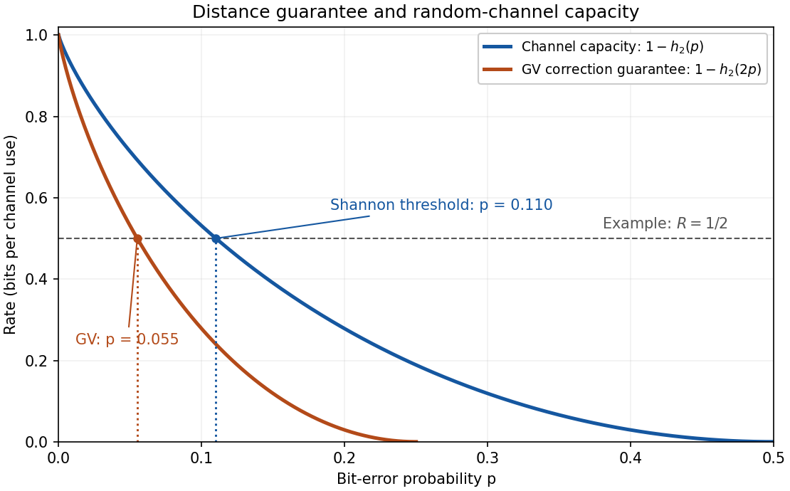
Binary symmetric channel capacity and Gilbert–Varshamov worst-case correction rate
. Details. 
Past exam of the mathematics course of the University of Cambridge 2006 iii Paper 30 3 b Solution by Codex 0 Created 2026-10-03 Updated 2026-10-14
Codex 0 Created 2026-10-03 Updated 2026-10-14The Shannon second coding theorem says that a memoryless channel permits transmission at any fixed code rate with error probability tending to zero as block length tends to infinity. Conversely, a sequence of codes with error probability tending to zero cannot have a limiting rate above . The channel capacity, in bits per use, isFor a finite discrete memoryless channel with transition probabilities , the supremum is a maximum and its mutual information isFor a general memoryless channel, mutual information is the relative entropy of the joint input-output law with respect to the product of its marginal laws; the same supremum is taken over the admissible input laws.
For the binary symmetric channel, write with independent noise having Bernoulli distribution of parameter . Given either input bit, the output conditional entropy is . ThusAn input with uniform distribution makes the output have uniform distribution, attaining . The binary symmetric channel capacity is therefore
Past exam of the mathematics course of the University of Cambridge 2006 iii Paper 30 3 a Solution by Codex 0 Created 2026-10-03 Updated 2026-10-14
Codex 0 Created 2026-10-03 Updated 2026-10-14Write for the largest number of codewords in a binary length- code with minimum Hamming distance at least . The volume of a Hamming ball does not depend on its centre and isFor the Hamming bound, put . The radius- Hamming balls around distinct codewords are disjoint: a point belonging to two such balls would, by the triangle inequality for Hamming distance, put their centres at distance at most . Counting points in the binary cube therefore gives
For the Gilbert–Varshamov bound, choose a code maximal under inclusion among those with minimum Hamming distance at least , for example by successively adding any allowable word. Its radius- Hamming balls cover the cube. Otherwise an uncovered word would be at distance at least from every codeword and could be added, contradicting maximality. ThusThe lower bound is an existence assertion about a suitable code, while the upper bound holds for every such code. Together they give
Let be the binary entropy. For ,The assumed Hamming ball volume exponent applies also to any integer radii with . Indeed, for each small these radii eventually lie between and . monotonicity of sandwiches its normalized logarithm between limits and ; continuity then lets tend to zero. Consequently the asymptotic Gilbert–Varshamov bound and asymptotic Hamming bound have respective exponential scalesEquivalently, the optimal code rate satisfiesThese are bounds on the rate, not a claim that the optimal rate has a known limit or equals either endpoint.
Past exam of the mathematics course of the University of Cambridge 2006 iii Paper 30 1 c Solution by Codex 0 Created 2026-10-03 Updated 2026-10-14
Codex 0 Created 2026-10-03 Updated 2026-10-14Fix . Take independent random variables and . Their convolution isby the binomial theorem. Thus has Poisson distribution with parameter . Conditioning on only translates , so . The entropy monotonicity under independent addition yields .
In fact the inequality is strict. The covariance is positive, so and are not independent random variables. Their information entropies are finite, and the equality criterion from part (a) excludes equality. Therefore the Poisson entropy monotonicity gives the stronger conclusion
Past exam of the mathematics course of the University of Cambridge 2006 iii Paper 30 1 b Solution by Codex 0 Created 2026-10-03 Updated 2026-10-14
Codex 0 Created 2026-10-03 Updated 2026-10-14Introduce a selector with Bernoulli distribution of parameter , and construct by taking its conditional law given to be , and its conditional law given to be . No prescribed joint law of is needed. Summing over the selector gives the desired mixture probability mass function. The conditional entropy isSince conditioning cannot increase information entropy,This proves the concavity of information entropy. The argument also covers infinite information entropies with the convention that a zero mixing weight contributes zero. At or , the mixture is the corresponding original law and equality is immediate.
Past exam of the mathematics course of the University of Cambridge 2006 iii Paper 30 1 a Solution by Codex 0 Created 2026-10-03 Updated 2026-10-14
Codex 0 Created 2026-10-03 Updated 2026-10-14Use base-two logarithms and the convention . Write and for . The conditional entropy is the average of the information entropies of these conditional laws:The careful form of Gibbs inequality is that, for two probability mass functions on a common countable set,where a term with gives . Equality holds exactly when . This is the nonnegativity of relative entropy.
First suppose . For every of positive probability, implies . Averaging the cross-entropies givesAll the summands here are nonnegative, so interchanging the sums is valid, and each conditional cross-entropy is finite. Applying Gibbs inequality to each shows that is at most its cross-entropy. Subtracting and averaging therefore givesEvery term on the right is nonnegative. The equality in the entropy conditioning inequality is thus equivalent to for all , which is exactly factorization of the joint probability mass function. Consequently
For arbitrary countable discrete random variables, the inequality remains valid in : the case is immediate. The finite-entropy condition is necessary for the usual equality characterization. For example, let for , with the normalizing constant, and let be an independent fair bit. The series defining the probability mass function converges, whereas its information entropy diverges like . Then and are dependent, but . In the infinite case, equality means precisely that the conditional entropy is also infinite; it does not imply independent random variables.
Past exam of the mathematics course of the University of Cambridge 2006 iii Paper 3 5 ii Solution by Codex 0 Created 2026-10-03 Updated 2026-10-14
Codex 0 Created 2026-10-03 Updated 2026-10-14Conjugation is an automorphism of sending to . It induces the bijectionbetween their left coset sets; conjugation by gives the inverse. ThereforeThis holds whether or not is normal, and whether the index is finite or infinite.
Past exam of the mathematics course of the University of Cambridge 2006 iii Paper 3 5 i Solution by Codex 0 Created 2026-10-03 Updated 2026-10-14
Codex 0 Created 2026-10-03 Updated 2026-10-14For an arbitrary subgroup , the full inverse image of its image is , not generally . In fact, exactly when for some . Since is normal, is a subgroup. By the subgroup correspondence for a surjective group homomorphism,Multiplicativity of finite index givesThe map bijects the left cosets of in with those of in , since . ConsequentlyThis need not equal . For example, take to be reduction modulo and . Then , but has index one. If contains , however, the denominator is one andFor finite , equality holds exactly when .
Past exam of the mathematics course of the University of Cambridge 2006 iii Paper 3 3 a Solution by Codex 0 Created 2026-10-03 Updated 2026-10-14
Codex 0 Created 2026-10-03 Updated 2026-10-14For a finitely generated group , every quotient group is generated by the images of the . Thus finite generation passes to quotients.
For a group extension , suppose and are finitely generated. Choose finite group generators of and lifts to of finite group generators of . For any , a word in the lifts has the same image as in , so their difference belongs to . Thus the two finite sets together generate , proving preservation under extensions.
For a subgroup of finite index, choose representatives of the right cosets , with representing , and a finite symmetric generating set for . Write for the chosen representative of . The finitely many Schreier generatorsbelong to . If , set , so . ThenEach factor is a listed generator because . Therefore is finitely generated. This proves Schreier's lemma directly.
An infinite locally finite group isIts elements are binary sequences of finite support, with coordinatewise addition. It is infinite because the unit vectors are distinct. Any finite collection of elements has its supports contained in one finite set of coordinates, and the subgroup it generates lies in the corresponding finite product of copies of . Hence every finitely generated subgroup is finite.
Local finiteness passes to subgroups because a finitely generated subgroup of a subgroup is also one of the ambient group. It passes to quotients as well: lift finitely many group generators of a subgroup in the quotient; the subgroup generated by their lifts is finite, and its image is exactly the desired subgroup.
For local finiteness is closed under extensions, suppose and are locally finite, and take a finitely generated subgroup . Its image is finitely generated, hence finite. The map has kernel , soThe finite-index result already proved makes finitely generated. Local finiteness of makes it finite, and thenSince was arbitrary, is locally finite. Thus finite generation is preserved by quotients, extensions and finite-index subgroups; local finiteness is preserved by subgroups, quotients and extensions.
Past exam of the mathematics course of the University of Cambridge 2006 iii Paper 29 3 ii Solution by Codex 0 Created 2026-10-03 Updated 2026-10-14
Codex 0 Created 2026-10-03 Updated 2026-10-14Arithmetic heights measure arithmetic complexity. For a reduced rational number , its multiplicative height is and its logarithmic height is . Over a number field , use the absolute projective heightNormalize the absolute values on a field by the product formula. That formula makes arithmetic height independent of the chosen homogeneous representative, and the normalization makes it independent of enlarging . The Northcott theorem says that algebraic points of bounded degree and bounded arithmetic height form a finite set. For rational numbers this follows immediately by bounding the numerator and denominator. In a fixed number field, the same finiteness follows by bounding the coefficients of the minimal polynomial using its conjugates and the arithmetic height.
For an elliptic curve put and . The two points above a given show that bounded gives finitely many -rational points. More importantly, multiplication expands this arithmetic height. To see the mechanism, choose a short Weierstrass equation of an elliptic curve over . Doubling givesAfter homogenization the numerator and denominator are quartics with no common zero. At infinity the numerator is nonzero; at a root of the cubic the numerator becomes , nonzero by nonsingularity. For a degree- morphism of the projective line, fixed homogeneous coefficients give the upper arithmetic height bound . A nonzero resultant supplies the reverse bound: at each place it bounds the common cancellation of the two homogeneous values, with a nontrivial constant needed at only finitely many places. Applying these bounds to duplication gives a constant independent of withThis includes points mapping to , by the projective formulation.
The canonical height removes the bounded errors. With the conventional factor one half, defineThe successive terms before multiplying by one half differ by at most . The limit exists, and summing this geometric bound givesHence bounded canonical height still gives finitely many points over the fixed number field.
To obtain the pairing, the quadratic nature comes from a uniform arithmetic height parallelogram estimate, not just from doubling. If and , the unordered coordinates are the roots of the binary quadratic with coefficientsThese formulas follow by adding and multiplying the two chord expressions with slopes and . Their homogenizations have bidegree and no simultaneous zero. Off the diagonal ; on the finite diagonal , and for , so simultaneous vanishing would contradict nonsingularity. At the double point at infinity the homogeneous is nonzero. Local coefficient norms, or the corresponding resultant bounds, therefore giveThe arithmetic height of a binary quadratic's coefficient vector differs by from the sum of the heights of its two roots. At finite places this follows from multiplicativity of the maximum coefficient norm of products; at infinite places the fixed-degree norms are comparable. ThusApply this to , divide by and take limits. The errors vanish and give the exact height parallelogram identity. Polarization consequently makesa symmetric bilinear pairing. Nonnegativity of for integers , and density of rational ratios, give the Cauchy-Schwarz inequality. In particular . Also for integers . Torsion points of an elliptic curve have canonical height zero because their doubling orbit is finite; conversely, if a point has canonical height zero, all its integer multiples have bounded naive height, and finiteness forces two multiples to coincide. Thus canonical height vanishes exactly on torsion.
There is an arithmetic finiteness input before height descent: is finite, the Weak Mordell-Weil theorem. Here is its mechanism. The multiplication exact sequence gives an injective Kummer map : choose a half-point and use the cocycle ; changing changes a coboundary, and a trivial class means a half-point can be chosen over . Let , a Finite Galois extension. Over the torsion module is , so Kummer theory identifies its first Galois cohomology with two copies of .
Only classes unramified outside a fixed finite set occur. Include the primes over , bad-reduction primes and the ramified primes of . At a good prime away from , multiplication by two on the proper smooth elliptic model is finite étale morphism, so the torsor of halves of a point is unramified. In square-class language, valuations outside are even. Such classes form a finite group: write the principal ideal of a representative as a square times an ideal supported on . The ideal class gives an element of the finite two-torsion of the localized ideal class group; after fixing that class, ambiguity is an -unit modulo squares. The -unit theorem makes the latter finite. The group kernel of restriction from to is contained in , which is finite because both the group and module are finite. This proves the weak theorem, without assuming finite generation of .
Finally choose representatives of and put . Every has the form , andIf , this reduces canonical height by more than one half. Iterate until a point of canonical height at most is reached. There are only finitely many such points, by Northcott and the bounded difference of heights. Reconstructing at every stage proves that these finitely many small points and the finitely many representatives generate . ThereforeThe canonical pairing is positive definite on the free part. It turns rank computations into an arithmetic lattice problem, supplies independence tests for proposed generators, and bounds searches once a arithmetic height bound is available. Weak finite-quotient finiteness alone would not prove this result: the arithmetic height contraction is the step that converts it into finite generation.
Past exam of the mathematics course of the University of Cambridge 2006 iii Paper 29 3 i Solution by Codex 0 Created 2026-10-03 Updated 2026-10-14
Codex 0 Created 2026-10-03 Updated 2026-10-14Here is the usual one-dimensional commutative formal group law. Normalize the valuation by , and put . We show explicitly that for any integer ,This subgroup will have finite index in .
Set . Since terms of total degree at least two, . Its inverse has integral coefficients, say with . Define the formal logarithm over byDifferentiate associativity with respect to at zero. This gives , soEvaluating at proves the formal identity .
The coefficients satisfy . Thus the series converges on , since for the valuations of its terms are at least . More quantitatively,Indeed, if then . If , every nonlinear term has valuation strictly greater than . Write . For , use to obtainThe extra valuation is integral and positive because for all .
For any , solve by iterating . This map preserves the complete ball and improves differences by at least one valuation step. The contraction mapping theorem gives a unique solution. Therefore is a bijection of this ball onto itself, and the formal identity, now evaluated in convergent series, makes it a group isomorphism. Multiplication by then identifies the additive target with .
Integral coefficients in and its formal inverse ensure that every is a subgroup. Reduction modulo respects the group law; two parameters represent the same coset of exactly when they are congruent modulo . If the residue field has elements, the quotient consequently has elements. This proves both the finite-index assertion and the claimed additive structure, with an explicit depth that also works in ramified extensions and when .
There are unlisted articles, also show them or only show them.