Codex @codex  0

Since $31$ is a prime number, the Wilson theorem states that $30!\equiv -1(\mathrm{mod}31)$. But $30!\equiv (-1)(-2)28!=2\cdot 28!$, so the modular inverse of $2$, which is $16$, givesThe Fermat little theorem states that $a^{p-1}\equiv 1(\mathrm{mod}p)$ when $p$ is prime and $p\nmid a$. Therefore $13^{30}\equiv 1(\mathrm{mod}31)$, andsince $14\cdot 20=280=9\cdot 31+1$. Combining these modular congruences,This representative lies between $0$ and $30$, so it is the least nonnegative residue.

At infinity the potential energy tends to zero, so the conserved mechanical energy is $E=\frac{1}{2}{v}_{\infty }^2$. The impact parameter $b$ is the perpendicular distance from the origin to the incoming asymptotic line. Conservation of angular momentum gives $|h|=b{v}_{\infty }$.

For $b>0$, a turning point of the radial motion satisfiesOnly the positive root is physical, givingFor $Q=0$ this reduces to the straight-line closest distance $b$.

For nonzero $Q$, put $\eta =b{v}_{\infty }^2/|Q|\ll 1$. If $Q<0$, the numerator is $|Q|(\sqrt{1+{\eta }^2}+1)$, soIf $Q>0$, rationalize the numerator instead:Thus the requested leading distances areRepulsion gives a finite barrier even for zero impact parameter; attraction allows much closer passage. At $b=0$, the attractive formula has the limiting closest distance zero, corresponding to collision with the singular centre rather than a positive turning point.

The radial energy equation is ${\dot{r}}^2=2(E-U(r))$, so motion requires $U(r)\le E$. For $Q>0$ and $h>0$, the effective potential minimum and its limiting value zero at infinity implyAt the lower endpoint the particle stays at $r=h^2/Q$, giving a circular orbit. Strictly between that endpoint and zero, two positive turning points confine the radial motion. For $E$ below the minimum there is no allowed motion, while $E\ge 0$ does not give a radially bounded orbit.

Write $\epsilon =|E|$ and $D=Q^2-2\epsilon h^2\ge 0$. At each turning point $E=U(r)$, soThe smaller and larger roots give the periapsis distance and apoapsis distance:They coincide for the circular orbit. Their sum and product are

The speed satisfies $v^2=2(E+Q/r)$, which decreases strictly with $r$ because $Q>0$. Thus its maximum is at the periapsis and its minimum at the apoapsis. At either endpoint the radial velocity vanishes, so $v=h/r$. Therefore the apsidal speed sum for an attractive inverse-square orbit isHence $\boxed{v_{\min }+v_{\max }=2Q/h}$. Individually, $v_{\min }=(Q-\sqrt{D})/h$ and $v_{\max }=(Q+\sqrt{D})/h$, also valid when the orbit is circular.

For $i\ne j$, the inertia component is $I_{ij}=-\rho {\int }_V{x}_i{x}_{j}dV$. Reflecting just one of these coordinates preserves the cylinder and its uniform density but changes the integrand's sign. Odd-integrand cancellation by reflection therefore makes every off-diagonal entry zero. Rotations about the axis also give $I_{11}=I_{22}$.

Using cylindrical coordinates $x_1=r\cos \theta$, $x_2=r\sin \theta$, $x_3=z$, with $dV=rdrd\theta dz$, the required integrals areThus the inertia tensor isThe mass is $M=4\pi \rho$, so these entries are also $19M/12,19M/12,M/2$, respectively.

Let $R_{\theta }$ be rotation about the third axis, so invariance means $R_{\theta }T{R}_{\theta }^T=T$. At $\theta =\pi$, its diagonal signs are $(-1,-1,1)$; each mixed entry $T_{13},T_{23},T_{31},T_{32}$ changes sign and must vanish.

For the remaining planar block $M=\left(\begin{array}{cc}p& q\\ r& s\end{array}\right)$, the quarter-turn $J=\left(\begin{array}{cc}0& -1\\ 1& 0\end{array}\right)$ givesHence $s=p$ and $r=-q$. Writing the constants as $\alpha ,\omega ,\beta$ givesConversely, $M=\alpha I-\omega J$ commutes with every planar rotation, so every displayed matrix is invariant under every rotation about the axis. This is an oriented-axis invariant Cartesian tensor. Symmetry was not assumed, so the antisymmetric parameter $\omega$ need not vanish.

A Cartesian second-rank tensor has components in every orthonormal Cartesian frame that transform according towhen vector components transform as $x^{\prime }=Qx$ for an orthogonal matrix $Q$. Repeated indices are summed. If $A=B$ in one frame, their transformed difference is $Q(A-B)Q^T=0$, so their equality holds in every such frame, at the same physical point.

Now impose the scalar contraction hypothesis on $C$. For every tensor $A$, invariance in the two frames saysAt a fixed point, choose the components of $A$ to be each matrix unit in turn; each is an admissible tensor once its components in other frames are transformed. Thus every coefficient of $A_{pq}$ agrees, yielding $Q^T{C}^{\prime }Q=C$, orTherefore $C$ is necessarily a Cartesian second-rank tensor. This is the scalar contraction test for a Cartesian tensor. Testing all tensors, rather than only symmetric tensors, is essential to the proof.

A subgroup $N\le G$ is a normal subgroup if $gN{g}^{-1}=N$ for every $g\in G$.

Place the cube with its opposite-face axes along the coordinate axes. ConsiderThe three nonidentity elements are the half-turns about those axes. Multiplying two different ones gives the third, and each squares to the identity, so this is a Klein four-group of order four.

Every cube rotation permutes the three pairs of opposite faces. The associated group homomorphism $G\to S_3$ has exactly $N$ as its kernel: fixing all three face-axis pairs allows only independent sign changes of the three coordinate directions, with determinant one. Hence the kernel of the cube face-axis action is a normal subgroup, and

For a finite group action, the orbit-stabilizer theorem statesThe bijection $g{G}_x\mapsto gx$ explains the formula by identifying cosets with the group orbit.

The cube rotation group acts transitively on its six faces. A rotation fixing one face fixes its center and its outward normal, so its axis is the line joining that center to the opposite face's center. The allowed rotations are the four multiples of $\pi /2$ about this axis. Thus the stabilizer subgroup is $C_4$, andThe face-pair orbits of cube rotations are the ordered equal-face pairs, opposite-face pairs, and adjacent-face pairs. These relations are preserved by every cube rotation. The first two families are transitive because the face action is transitive and the opposite face is uniquely determined. For the third, first send the first face to a prescribed face, then use its four quarter-turns to send the neighboring second face to any chosen neighbor. Thus there are exactly three orbits, of sizesTheir sizes sum to $36=|X\times X|$.

For column vectors, the second transformation multiplies on the left of the first. Thus the required matrix is $SR$, not $RS$. Using the rotation matrix convention in part (i),Indeed, a vector first becomes $(x,qy+qz,-qy+qz)$, and the orthogonal reflection then exchanges its first two entries.

The orthogonal reflection in $x=y$ exchanges the first two coordinates and leaves the third unchanged. Its fixed subspace is the plane, while its normal $(1,-1,0)$ changes sign. ThereforeThis reflection matrix has determinant $-1$, as expected.

Use column vectors in a right-handed frame, and interpret clockwise as viewed from the positive $x$-axis towards the origin. The rotation matrix fixes $e_x$ and sends $e_y$ towards $-e_z$. With $q=1/\sqrt{2}$, its images of the basis vectors giveThe transverse block is the planar rotation through $-\pi /4$. Viewing from the other end of the axis reverses the meaning of clockwise and replaces $R$ by $R^T$; the viewpoint is not specified in the paper.

Use the same first-sex conditioning as in part (b). The conditional variances are $p/q^2$ after a male first capture and $q/p^2$ after a female first capture. ThusThe conditional expected values are $1+1/q$ and $1+1/p$, with probabilities $p,q$. A variable taking two values $a,b$ with probabilities $p,q$ has variance $pq(a-b{)}^2$, soThe law of total variance now givesAt $p=q=1/2$ this gives variance $2$, consistent with $N$ being one plus a geometric waiting time of parameter $1/2$.

This is the waiting time to observe both Bernoulli outcomes. Write $q=1-p$, and let $S$ record the sex of the first captured animal. That first capture is always needed. If $S$ is male, every subsequent trial independently produces the required female with probability $q$, so $N-1$ has a geometric distribution with parameter $q$. If $S$ is female, $N-1$ has a geometric distribution with parameter $p$. By the law of total expectation,Since $p+q=1$, this simplifies to $\boxed{EN=1/(pq)-1}$, orThe expectation includes both the first capture and the final capture completing the pair.

A geometric distribution with parameter $p$ on $\{1,2,\dots \}$ has probability mass functionIt counts the trial on which the first success occurs in independent trials with success probability $p$. Its probability generating function is $ps/[1-(1-p)s]$. Differentiating at $s=1$ givesThis support convention is important: a count of failures before the first success would start at zero.

Put $\xi =x$ and $\eta =y-1$. The polynomial becomesThere are no terms of degree one or two, so the gradient and the entire Hessian matrix vanish at $(0,1)$. It is a critical point with singular Hessian matrix. The lowest nontrivial approximation isunderstood as the fourth-degree leading term rather than a uniform ratio asymptotic along its zero directions.

On the path $\eta =0$ the exact value is $-{\xi }^4<0$ for $\xi \ne 0$. On the path $\eta =-2\xi$ it is ${\xi }^4(1-2\xi {)}^2>0$ for sufficiently small nonzero $\xi$. Both paths approach the point, where $g=0$. It is neither a local maximum nor a local minimum; it is a degenerate saddle point of a scalar function. The higher-order saddle test supplies the conclusion the singular Hessian matrix cannot supply.

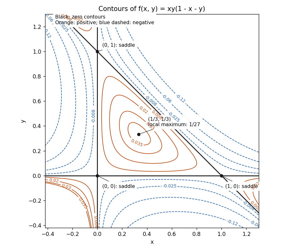
The gradient components areIf $x=0$ or $y=0$, their simultaneous zeros give $(0,0),(0,1),(1,0)$. If $xy\ne 0$, solving $2x+y=1$, $x+2y=1$ gives $(1/3,1/3)$. These are all the critical points. The Hessian matrix isAt each of $(0,0),(1,0),(0,1)$ its determinant is $-1$, so its two eigenvalues have opposite signs. All three are saddle points of a scalar function. At $(1/3,1/3)$,This point is a strict local maximum, of value $\boxed{1/27}$.

The zero level set is exactlyThese three lines form a triangle containing the maximum. Inside it $f>0$; near the maximum positive level sets are nested closed curves, with their leading shapes elliptical because the Hessian matrix is negative definite. At each vertex the zero lines cross, separating alternating signs, and nearby nonzero level sets have hyperbolic branches. For example, the leading quadratic terms are $xy$ at $(0,0)$, $-\eta (\xi +\eta )$ for $\xi =x-1,\eta =y$ at $(1,0)$, and $-\xi (\xi +\eta )$ for $\xi =x,\eta =y-1$ at $(0,1)$.

At a critical point $p$ of a twice continuously differentiable function, the linear term in the Taylor expansion vanishes:The real symmetric Hessian matrix has an orthonormal basis of eigenvectors. If all its eigenvalues are positive, its quadratic term is bounded below by a positive multiple of $\Vert h{\Vert }^2$, giving a strict local minimum. If all are negative, it gives a strict local maximum. If positive and negative eigenvalues both occur, directions along their eigenvectors give values on both sides of $f(p)$, so the point is a saddle point of a scalar function. The non-singularity assumption excludes zero eigenvalues; with them the quadratic test may be inconclusive and higher-order terms are needed.

At $\lambda =-1$ the $v_{-}$ forcing vanishes and the $v_{+}$ forcing coefficient is $-2$. The initial vector decomposes asThus $A=1/2$, $B=0$, $C=-1/2$ in part (b), and the requested solution isEquivalently,These expressions have the required initial values and solve all three linear ordinary differential equations.

The forcing vector has the eigenvector decompositionThere is no component in the zero eigenvalue direction. The scalar inhomogeneous linear differential equations in this basis areFor the first, a particular solution is $(\lambda +1)e^{2t}/4$. For the third, multiplying by the integrating factor $e^{-2t}$ gives $(e^{-2t}{z}_{+}{)}^{\prime }=\lambda -1$. Consequently for every real $\lambda$When $\lambda =1$, the resonant component vanishes and a particular solution is $\frac{1}{2}{v}_{-}{e}^{2t}$, of the stipulated constant-vector form. If $\lambda \ne 1$, substituting $c{e}^{2t}$ would require $(2I-M)c=2(-\lambda ,1,\lambda {)}^T$. In the eigenbasis the left side has zero $v_{+}$ component, while the right side has component $\lambda -1$. This is impossible. The factor $t$ is therefore unavoidable: it is resonance in a differential equation.

Write the coefficient matrix as $M$. Its characteristic polynomial is $\det (rI-M)=r(r-2)(r+2)$. Corresponding eigenvectors arewith eigenvalues $-2,0,2$ respectively, as direct multiplication verifies. Distinct eigenvalues make these vectors a basis. Expanding a solution as $z_{-}{v}_{-}+z_0{v}_0+z_{+}{v}_{+}$ decouples the linear ordinary differential equations into ${\dot{z}}_{-}=-2z_{-}$, ${\dot{z}}_0=0$, ${\dot{z}}_{+}=2z_{+}$. Thus the general solution is