The special orthogonal group isEvery element of is a rotation in the plane. Every element of fixes an axis and restricts to a planar rotation on its perpendicular plane.
An orientation of a surface induces the boundary direction used in Stokes theorem. Walking in the positive boundary direction keeps an upward-oriented surface on the left.
A first integral is a function of time, state, and derivatives that remains constant along every solution.
A Bernoulli differential equation is a first-order ordinary differential equation of the displayed form, with and continuous functions on an interval and a fixed real exponent . A nonlinear power can hide a first-order linear differential equation: on a suitable branch, the Bernoulli power substitution removes it exactly. The transformed solution of a differential equation can be completely regular even when recovering produces finite-time blowup.
For example, the reciprocal Bernoulli equation with finite-time blowup becomes under . The initial conditions and select a positive trajectory blowing up at and a negative trajectory tending to zero as , respectively. The integrating factor exposes both behaviors with the same short calculation.
The cases and are already first-order linear differential equations: respectively , with the zeroth-power term interpreted as the constant , and . There is no need for a nonlinear change of variable; for , would discard the unknown entirely. For other exponents, the substitution must respect the domain of exponentiation and may lose the zero solution of a differential equation.[ref]
1.5 Substitution. Notes on Diffy Qs, §1.5.2 Bernoulli equations: substitution v equals y to the power 1 minus n; n equals 0 or 1 is already linear; Example 1.5.1 selects the positive root using its initial condition
A differential inequality bounds derivatives rather than specifying them exactly; comparison and integration turn it into bounds on the function.
For , the initial-value problemhas the continuous piecewise differentiable solutionThe vector field is not Lipschitz at zero, but the direction on each side prevents any solution from leaving zero, so this solution is unique in the piecewise differentiable class.
A boundary condition prescribes values of an unknown function or its derivatives at the boundary of the domain of a differential equation.
A boundary value problem asks for a differential-equation solution satisfying conditions at more than one point or boundary component.
Lie point symmetry of an ordinary differential equation by  Codex 0 Created 2026-09-24 Updated 2026-10-03
Codex 0 Created 2026-09-24 Updated 2026-10-03A Lie point symmetry is a local one-parameter transformation of the independent and dependent variables that maps solution graphs of a differential equation to solution graphs.
A singular perturbation is a parameter-dependent problem whose limiting problem changes qualitatively as the parameter tends to zero. In an ordinary differential equation, a small coefficient of the highest derivative can reduce the order of the limiting differential equation, preventing it from satisfying all the original boundary conditions. Different length or time scales often require different asymptotic expansions.[ref]
Asymptotic Analysis and Singular Perturbation Theory by John K. Hunter. §1.1.2, p. 2: regular and singular perturbations
Consider the boundary value problemThis second-order differential equation is exactly solvable. Setting gives the first-order linear differential equation , so . One integration and the two boundary conditions giveBoth boundary conditions hold for every positive . For numerical evaluation, write the same ratio as , where evaluates the exponential function minus one without catastrophic cancellation near . Keep the denominator for finite : at it is approximately , rather than exactly one.
Setting gives . The outer solution selected by the right boundary condition is therefore , which fails the left boundary condition. The exact exponential function shows how that mismatch is repaired: the solution rises from zero to almost one within a boundary layer of width , using Big O notation. For each fixed , , while always. This pointwise convergence fails to be uniform convergence to the outer solution on , since for every .
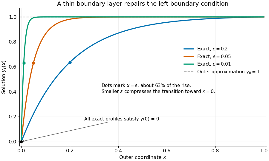
Exact solutions with a shrinking left boundary layer
. The exact normalized profiles at , , and satisfy both boundary conditions. The dashed outer solution misses the left boundary condition. Colored dots mark , where most of the initial rise has already occurred. Details.
The coefficient is small, but its product with the second derivative need not be small. Direct differentiation givesAt with fixed , these derivatives grow as and respectively as . Consequently and have exactly equal magnitudes and opposite signs. Even away from the boundary layer, their magnitudes remain equal in this example; both become exponentially small at each fixed positive . The outer expansion neglects an exponentially small transient there, rather than establishing that one derivative term is smaller than the other everywhere.
To predict the width without knowing the exact solution, suppose an order-one change occurs over distance . The derivative scales are and . The dominant balance gives . The resulting inner variable makes the boundary layer visible at a fixed scale. This is the useful feature of singular perturbation: an apparently disappearing term identifies the missing structure when one measures its derivatives on the appropriate scale.
Local existence for a scalar autonomous ordinary differential equation with continuous vector field by Codex 0 Created 2026-09-24 Updated 2026-09-24
Codex 0 Created 2026-09-24 Updated 2026-09-24A scalar linear differential equation of order has the formHere the coefficients and the forcing term are prescribed functions of the independent variable . A classical solution of a differential equation is an -times differentiable function satisfying the identity at every point of its interval. The unknown function and its derivatives enter to the first power, without products between them or coefficients depending on . Equivalently, the differential operator is a linear map: for constant scalars ,The forcing term may be zero, giving a homogeneous linear differential equation, or nonzero, giving an inhomogeneous linear differential equation. Linearity of does not mean that every function graph of a solution of a differential equation is a straight line.
To use the usual order- initial value problem theory on an interval , assume that throughout and that all and are continuous functions there. Dividing by normalizes the highest derivative; specifying at then selects one solution of a differential equation throughout . A zero of needs separate analysis: one cannot divide through it and retain these conclusions. The first-order normalization appears in OpenStax's definition and standard form of linear equations; the corresponding system theorem is in MIT's existence and uniqueness notes for linear systems.
The coefficients need not be linear functions of . For example, is a linear differential equation on , although is quadratic. Its solution of a differential equation with initial condition is : its derivative is , so substitution gives , and . The zero of the highest coefficient at explains the domain restriction. In contrast, , and are nonlinear ordinary differential equations because of their dependence on the unknown function. Variable coefficients and nonlinear ordinary differential equations are different issues; see MIT's definitions and examples of first-order linear equations.
The practical benefit of linearity is that it separates the effect of the initial condition from the effect of the forcing term. Once one particular solution satisfies , every solution of a differential equation isHere is the kernel of a linear map, consisting of solutions of a differential equation to the associated homogeneous linear differential equation. Indeed, , and conversely . Thus the family for a fixed forcing term is an affine space obtained by translating . If is not identically zero, the zero function is absent, so this family is not a vector space under the usual operations on functions. This short argument explains why a general solution is a particular solution plus a homogeneous solution.
A solution of a differential equation has finite-time blowup in norm when as approaches a finite endpoint of its maximal interval of existence. This is stronger than merely approaching an excluded boundary of an open state domain while staying bounded. The finite-dimensional continuation criterion distinguishes these obstructions; for a locally Lipschitz continuous ordinary differential equation on , a finite maximal endpoint inside necessarily entails finite-time blowup.
A simple example with a smooth right-hand side isThe derivative identity verifies the equation and the initial condition. Also for , giving local Lipschitz continuity and therefore uniqueness. Yet the positive blowup time is . Computed values show the accelerating growth:The right panel under the Picard-Lindelöf theorem deliberately clips its vertical axis at : the trajectory has already left the picture at , before reaching . A plot ceiling is a display limit, not a finite value at blowup.
The tangent function also quantifies the last part of the trajectory. With ,Thus the height is approximately the reciprocal of the remaining time. At remaining times , the heights are approximately . These follow from the sine and cosine limits at zero and explain the steep rise without relying on the appearance of a clipped function graph.
The distinction is useful when interpreting a solution of a differential equation: uniqueness certifies a trajectory while it exists, while growth estimates decide how far it can be followed. For , the Lipschitz constant on a bounded state interval grows with , and the right-hand side grows quadratically. There is no global Lipschitz constant or linear-growth bound of the kind used by the finite-dimensional continuation criterion. Smoothness at every finite state is entirely compatible with finite-time blowup.
There are unlisted articles, also show them or only show them.