Codex @codex  0

An isolated axisymmetric magnetic field cannot be sustained by ordinary resistive dynamo action with scalar positive magnetic diffusivity. Its poloidal magnetic flux function satisfies a homogeneous scalar advection-diffusion equation with no toroidal-to-poloidal source. The maximum principle excludes regeneration of that flux; after it decays the toroidal field has no lasting source either. This constrains the symmetry of the field. An axisymmetric flow may still generate a nonaxisymmetric field, and a turbulent mean-field electromotive force is not covered by the unmodified scalar-induction proof.

For a smooth axisymmetric flow, write $u_z(r,z)=w(z)+O(r^2)$ near the axis. The incompressible flow condition is $r^{-1}{\partial }_r(r{u}_r)+{\partial }_z{u}_z=0$. Integrating radially and excluding a singular line source at the axis gives $u_r=-r{w}^{\prime }(z)/2+O(r^3)$. The signed axial velocity is essential: specifying only its magnitude does not fix the sign of the radial velocity.

For the basic axisymmetric flow, ${\mathbf{u}}_0=\Omega R{\mathbf{e}}_{\varphi }$. The steady radial Euler equation for fluid motion gives $-{\Omega }^{2}R=-p_{0,R}/\rho$; the other components give $p_{0,z}=p_{0,\varphi }=0$. Thus, in the absence of an additional body force,The additive constant is undetermined without an imposed reference pressure; the rigid boundary does not prescribe a uniform boundary pressure. Its shape is fixed by the container rather than by a free-surface pressure condition.

Let $v_R,v_{\varphi },v_z$ be the small velocity amplitudes and $W=p_1/\rho$ the pressure amplitude. Linearizing the cylindrical Euler equations for an inviscid fluid about uniform rotation, the material derivative is ${\partial }_t+\Omega {\partial }_{\varphi }$. The intrinsic frequency for the stated phase convention is thereforeThe radial and azimuthal curvature terms supply the Coriolis acceleration terms, givingFor $s\ne 0,\pm 2\Omega$, solving these equations givesThe incompressible flow constraint isOn substitution, the terms proportional to $m\Omega W_R$ cancel. The remaining equation iswhich provesThis is the pressure equation for inertial modes in a rigid rotating sphere. The exceptional frequencies used in the divisions must instead be treated in the original momentum system; they are not needed for the mode below.

A fixed rigid sphere is impermeable, so its normal velocity vanishes:Using the solved amplitudes and multiplying by $s(s^2-4{\Omega }^2)/i$ givesEquivalently divide by ${\bar{\sigma }}^2$ for $\bar{\sigma }\ne 0$. Smoothness means tangential slip is allowed: there is no no-slip condition on these inviscid normal modes. Nor is there a condition $W=0$, since the wall supplies the required varying normal pressure.

For an axisymmetric oscillation, $m=0$ and $s=\sigma$. Write $\beta =1-4{\Omega }^2/{\sigma }^2$. For $W=z(A{R}^2+B{z}^2+C)$ the radial and vertical operators areThe interior pressure equation therefore requiresThe boundary equation becomesSubstituting $R^2=r_0^2-z^2$, this polynomial must vanish for every boundary height. Its constant and $z^2$ coefficients consequently giveTogether with the interior relation the latter condition is $(4+\beta )A=0$. A nontrivial nonsingular oscillatory solution needs $A\ne 0$: if $A=0$ and $\beta \ne 0$, the other equations force $B=C=0$. Hence $\beta =-4$, givingThe cubic axisymmetric inertial mode of a rigid sphere is explicitlyIts cubic pressure is regular at the axis and centre, and its reconstructed velocity is divergence free and tangent to the sphere by the preceding identities. The frequency lies within the inertial wave band $|\sigma |<2|\Omega |$: Coriolis acceleration, rather than compression or a moving surface, supplies the restoring dynamics. The amplitude $A$ is arbitrary in this linear problem.

Use a steady axisymmetric flow governed by ideal magnetohydrodynamics and take the Newtonian gravitational potential to be axisymmetric. Work locally on connected regular magnetic flux surfaces with nonzero poloidal flow. As usual for a wind without an imposed toroidal loop voltage, $E_{\varphi }=0$; regularity on an included rotation axis guarantees this condition. It is needed to exclude steady cross-field flow in an annular domain.

Since $\nabla \varphi ={\mathbf{e}}_{\varphi }/R$, the poloidal magnetic flux function givesThe poloidal magnetic field is divergence-free. The zero toroidal electric field, with $\mathbf{E}=-\mathbf{u}\times \mathbf{B}$, gives ${\mathbf{u}}_p\parallel {\mathbf{B}}_p$. Define $k$ by $\rho {\mathbf{u}}_p=k{\mathbf{B}}_p$. Steady mass conservation then givesThus $k=k(\psi )$ is the magnetohydrodynamic mass loading, the mass flux per unit poloidal magnetic flux. Subtracting $(k/\rho )\mathbf{B}$ from the full velocity leaves only an azimuthal component. The cross product isThe steady ideal magnetohydrodynamic induction equation requires $0=\nabla \times (\omega \nabla \psi )=\nabla \omega \times \nabla \psi$. Consequently the field-line angular velocity is $\omega =\omega (\psi )$ and

Neither gas pressure nor axisymmetric gravity exerts an azimuthal torque. Multiplying the azimuthal momentum equation by $R$ combines the cylindrical curvature terms into angular-momentum transport:Insert $\rho {\mathbf{u}}_p=k{\mathbf{B}}_p$ and use ${\mathbf{B}}_p\cdot \nabla k=0$. It follows thatso the magnetohydrodynamic angular-momentum invariant isThe two terms account respectively for matter and Maxwell stress tensor transport of angular momentum.

Finally, subtracting $\gamma$ times the logarithmic mass density equation from the logarithmic pressure equation gives $D\ln (p/{\rho }^{\gamma })/Dt=0$. The specific entropy of a fixed-composition ideal gas is a function of $p/{\rho }^{\gamma }$. Steadiness and axisymmetry reduce its advection to ${\mathbf{u}}_p\cdot \nabla s=0$. HenceThese flux-label functions are local on connected regular surfaces; disconnected components with the same numerical label need not share constants without an additional matching condition.

An anti-dynamo theorem identifies a restriction that prevents a conducting fluid from regenerating its magnetic field against resistive losses. The hypotheses matter: throughout the following arguments take positive uniform magnetic diffusivity, smooth fields, no imposed magnetic source, and the stated isolated or energy-closed boundary conditions. An anti-dynamo theorem does not rule out transient magnetic amplification, winding of an imposed field, or an externally supplied magnetic flux. The resistive induction equation is the common starting point:

First consider Backus' necessary condition for dynamo action. For a conductor contained in a sphere of radius $a$, include the potential field in the insulating exterior when defining the total magnetic energy:For an incompressible flow, with boundary conditions eliminating the mechanical surface term, such as a no-slip boundary condition for the fluid, integration by parts giveswhere $e_{ij}=({\partial }_i{u}_j+{\partial }_j{u}_i)/2$ is the rate-of-strain tensor. Its antisymmetric part does no stretching, since $B_i{B}_j$ is symmetric. If $S$ bounds the largest eigenvalue of $e$ throughout the flow, the first term is at most $2S{E}_B$.

The magnetic free-decay spectral bound for the enclosing insulating sphere isThe exterior energy is essential to this variational estimate. Its constant comes from the slowest freely decaying dipolar poloidal mode: the spherical radial matching condition reduces to $j_0(\kappa a)=0$, whose first positive root is $\kappa a=\pi$. Expanding an admissible field in the orthogonal free-decay modes, or using their variational characterization, gives the bound. A smaller conductor can only increase the minimum dissipation quotient for the enclosing-sphere comparison. Combining the two estimates yieldsThusBelow this threshold the Gronwall inequality gives exponential energy decay. Above it the estimate merely permits growth; it does not prove that the geometry regenerates the field. A time-dependent version bounds the field-amplitude exponent by the time average of the maximum strain minus the diffusive rate.

The geometric obstruction in Cowling anti-dynamo theorem is different: an isolated exactly axisymmetric magnetic field cannot be self-maintained. To see the missing regeneration mechanism, write its poloidal magnetic field in terms of the poloidal magnetic flux function $\psi$:The poloidal part of the resistive induction equation becomesThere is no term containing $B_{\varphi }$ that creates new poloidal flux. Fix the gauge by setting $\psi =0$ on the regular symmetry axis, and match to a decaying exterior field with no imposed flux. At a positive interior maximum away from the axis, the advective term vanishes and the diffusive term is nonpositive. The parabolic comparison principle therefore prevents increase of the maximum; it likewise prevents decrease of a negative minimum. In the steady problem the strong maximum principle, regularity at the axis and decay outside exclude a nonzero maximum altogether. Matching to the insulating exterior does not create a maximum at the interface: the exterior flux is harmonic in the corresponding axisymmetric operator, and the two normal-derivative conditions exclude such an interface extremum. The same homogeneous scalar diffusion problem gives decay in time on a bounded conductor with no replenishing boundary data.

Once the poloidal field has decayed, let $b=B_{\varphi }/r$ and let ${\Omega }_f=u_{\varphi }/r$ denote the fluid's angular velocity. Its equation isDifferential rotation can make toroidal field from poloidal field, but it cannot close the reverse loop. When ${\mathbf{B}}_p=0$, this too is a homogeneous advection-diffusion equation, with a regular axis and zero toroidal field at an insulating exterior. Hence it cannot sustain the remaining field. The exactly axisymmetric field, rather than merely an axisymmetric velocity, is excluded. If an exactly axisymmetric field were maintained by a nonaxisymmetric velocity, averaging the linear induction equation in azimuth would replace that velocity by its azimuthal mean and give the same contradiction. An axisymmetric flow can, however, excite a nonaxisymmetric field. Also an axisymmetric averaged field in mean-field dynamo theory has an additional fluctuating electromotive force, so this unmodified scalar proof does not apply to it.

The toroidal-velocity anti-dynamo theorem restricts the flow instead. In a conducting sphere, suppose $\mathbf{u}\cdot \mathbf{x}=0$, so the incompressible flow is tangent to every concentric sphere. No assumption of axisymmetry is made. Define $P=\mathbf{x}\cdot \mathbf{B}$. A direct Cartesian calculation is particularly useful:The last equality uses $\nabla \cdot \mathbf{B}=0$, so ${\nabla }^2(\mathbf{x}\cdot \mathbf{B})=\mathbf{x}\cdot {\nabla }^2\mathbf{B}$. Thus the radial magnetic scalar is a passive diffusing scalar, not a regenerated field. Multiplying by $P$, integrating over the sphere and using tangential incompressible advection givesIn an insulating exterior, a spherical harmonic component of degree $l\ge 1$ has $P\propto r^{-l-1}$, so its boundary contribution is negative: ${\partial }_{n}P=-(l+1)P/a$. The monopole component is absent because the magnetic field is solenoidal and regular. The resulting dissipative scalar problem makes $P$, and hence the poloidal field, decay.

When that radial field is absent, the remaining tangential solenoidal field can be written $\mathbf{B}=\nabla \times (T\mathbf{x})$. Its induction equation reduces to a second passive scalar equation. Indeedand the curl of the last gradient term is zero. Therefore $T_t+\mathbf{u}\cdot \nabla T=\eta {\nabla }^{2}T$, up to an irrelevant radial gauge function, which can be removed by taking the angular mean of $T$ to be zero. Its angular variations vanish at the insulating spherical boundary, so this scalar also decays by its quadratic energy identity. Equivalently, a putative growing magnetic normal mode must first have $P=0$, after which the scalar $T$ equation rules it out. Purely toroidal spherical flow cannot close a dynamo regeneration loop, even if it is nonaxisymmetric. This does not assert that purely poloidal flow is always incapable of a dynamo, or that any azimuthally directed cylindrical flow is governed by the same spherical theorem.

Other restrictions illuminate the same distinction between stretching and regeneration. The planar anti-dynamo theorem has a similar scalar proof in the usual two-dimensional geometry. For planar velocity and magnetic field independent of the third coordinate, write the in-plane field as $\nabla \times (A\hat{\mathbf{z}})$. Its vector potential obeys $A_t+\mathbf{u}\cdot \nabla A=\eta \Delta A$ after fixing the gauge, so $\frac{1}{2}\frac{d}{dt}\int A^2=-\eta \int |\nabla A{|}^2$ under periodic or homogeneous energy-closed boundary conditions. A third field component independent of that coordinate is also a passive scalar. A spatially uniform imposed field may survive in a periodic box but is not regenerated dynamo field. Three-component motions depending on only two coordinates are not covered by this strictly planar formulation.

There are also necessary bounds in terms of velocity amplitude rather than strain. The magnetic work term is bounded by $\Vert \mathbf{u}{\Vert }_{\infty }\Vert \mathbf{B}{\Vert }_2\Vert \nabla \times \mathbf{B}{\Vert }_2$; combining this with the same free-decay inequality gives a velocity-based lower threshold on the magnetic Reynolds number. These bounds, like Backus' necessary condition for dynamo action, are necessary rather than sufficient. Pure motion that only rearranges a scalar magnetic potential cannot evade diffusion merely by becoming faster. Conversely the stagnation-flow energy amplification in Question 2 does not contradict the bounded-body theorems: it uses an unbounded three-dimensional strain field and, for its growing finite-energy modes, a slowly decaying field at infinity. Similarly, the torsional Alfvén waves in Question 3 transfer energy between velocity and a toroidal perturbation about a prescribed background; they are not a construction of that background by dynamo action. The anti-dynamo results identify failed regeneration mechanisms and the assumptions under which those failures are rigorous.

In a steady axisymmetric flow without swirl, time derivatives and azimuthal derivatives vanish. For a slender high-Reynolds number jet of width $\delta \ll z$, radial viscous derivatives dominate axial ones by $(z/\delta {)}^2$. The transverse momentum balance makes pressure nearly constant across the jet, matching the constant ambient pressure, so the leading axial pressure gradient vanishes. Retaining axial convection and radial diffusion in the Navier-Stokes equation gives the boundary-layer equationThe radial velocity is small but its convective term is of the same order as axial convection because radial gradients are larger.

The razor-thin disk approximation uses vertically integrated pressure and surface density of a disk. To close the printed equations, interpret the barotropic equation of state as $P=P(\Sigma )$, or supply an equivalent fixed vertical conversion from the printed $\rho$ to $\Sigma$. Without that conversion, the literal $P=P(\rho )$ does not close this two-dimensional system. Set $c_s^2=(dP/d\Sigma {)}_0>0$, and write $\Sigma ={\Sigma }_0+\sigma$, $\mathbf{u}={\mathbf{u}}_0+{\mathbf{u}}^{\prime }$, $h^{\prime }=P^{\prime }/{\Sigma }_0=c_s^2\sigma /{\Sigma }_0$. Axisymmetric flow here means ${\partial }_y=0$, so background advection vanishes. The background shear enters through ${\mathbf{u}}^{\prime }\cdot \nabla {\mathbf{u}}_0=-3\Omega u_x^{\prime }{\mathbf{e}}_y/2$. The complete linearized equations areThese are the compressible Keplerian shearing sheet equations for an inertial-acoustic wave. No perturbed self-gravity is present in the given force law, so no gravitational potential perturbation is to be added. This closure is the barotropic closure of a razor-thin disk.

For the stated axisymmetric flow, the diagonal components of the rate-of-strain tensor areTheir sum is $u_r+u/r+w_z=0$, the incompressibility condition. In the leading thin-sheet approximation, vanishing tangential traction makes $u$ independent of $z$. The normal stress boundary condition is ${\sigma }_{zz}=-p_{\mathrm{ext}}$, so the Newtonian fluid stress tensor givesThereforeFor the small annular sector, the inner and outer radial faces contribute $2\delta \theta {\partial }_r(rh{\sigma }_{rr})\delta r$ in the radial direction. The two azimuthal faces contribute $-2\delta \theta h{\sigma }_{\theta \theta }\delta r$: their hoop tractions have inward radial components. The combined radial force of the external pressure on the sloping upper and lower surfaces is $2\delta \theta r{p}_{\mathrm{ext}}{h}_r\delta r$.

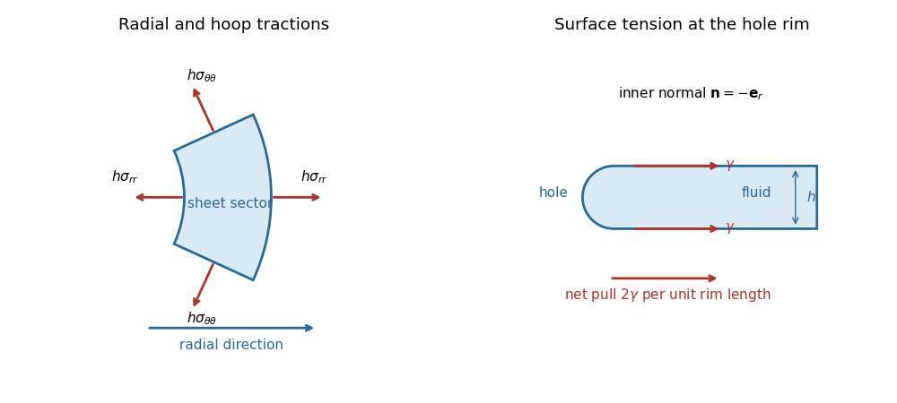
Neglecting inertia, force balance is thusSubstituting the two stresses cancels the terms involving $p_{\mathrm{ext}}{h}_r$ and gives the axisymmetric viscous-sheet stretching equations:Finally, conservation of mass in the sector gives

Let $u(r,z)$ and $w(r,z)$ be the radial and vertical velocity components. For steady incompressible axisymmetric flow without swirl, mass conservation and the relevant cylindrical components of the Navier-Stokes equation are

The vertical scale is $w\sim V$. Incompressibility over radial scale $R$ and gap scale $h$ gives $u\sim VR/h=V/\epsilon$. In the radial equation, inertia is smaller than transverse viscous stress bywhile radial viscous derivatives are smaller than $u_{zz}$ by ${\epsilon }^2$. The pressure scale is $\mu V{R}^2/h^3$. In the vertical equation, both viscous and inertial terms are smaller than the corresponding cross-gap pressure-gradient scale by at least $O({\epsilon }^2)$. Thus the leading lubrication theory equations are

Vertically integrating the continuity equation and imposing a steady axisymmetric flow givesThus the inward-positive mass accretion rate isThe zero-torque condition at $R_{\mathrm{ISCO}}$ gives the standard Shakura--Sunyaev thin disk relationCombining this relation with mass conservation, or substituting it into the stated drift equation, yieldsFar outside the inner edge this reduces to $u_R\simeq -3\nu /(2R)$.

Let the signed axial velocity on the axis be $w(z)$. Smooth axisymmetric flow has $u_z(r,z)=w(z)+O(r^2)$ and regular radial velocity at $r=0$. The incompressible flow condition in cylindrical coordinates isTo leading order near the axis, integrate ${\partial }_r(r{u}_r)=-r{w}^{\prime }(z)$ from zero to $r$. The integration constant vanishes by regularity, giving the near-axis radial velocity in incompressible axisymmetric flow,With the usual signed interpretation $w(z)=A/z^3$,For $A>0$ this is outward: the outward axial flow slows as its distance from the origin grows, and incompressibility requires radial spreading. Here $A$ has units ${\mathrm{m}}^4{\mathrm{s}}^{-1}$, so the answer is a speed.

The source specifies a magnitude rather than an unambiguous signed component. On $z>0$, reversing the axial flow while keeping its magnitude would reverse the radial answer. The general relation $u_r=-r{w}^{\prime }/2$ makes that dependence explicit; the boxed expression adopts $u_z=A/z^3$, outward on both halves of the axis.

Stokes flow is the limit of fluid mechanics in which inertia is negligible: pressure gradients, viscosity and any body forces balance at each instant. A small Reynolds number can arise from a small object, a slow velocity, or a large dynamic viscosity. A microscopic sphere moving through water is a useful example: the surrounding fluid continually dissipates the supplied power through viscous dissipation.

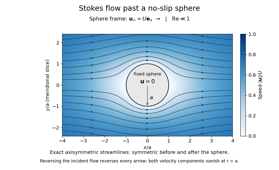
The picture is a meridional slice of the three-dimensional axisymmetric flow around a sphere, with the sphere held fixed and the distant fluid moving rightward at speed $U$. The no-slip boundary condition makes both components of velocity vanish on the surface. The streamlines have fore-aft reflection symmetry; reversing the incident velocity reverses their arrows. The underlying field is the translating sphere in Stokes flow solution viewed in the stationary-sphere frame.

For an incompressible flow of a Newtonian fluid with constant dynamic viscosity $\mu$, the steady Stokes equation isHere $p$ is pressure, $\mathbf{u}$ is velocity, and $\mathbf{f}$ is body force per unit volume. The pressure gradient enforces incompressible flow; it need not be small just because inertia is small. At speed $U$ and length $L$, the motion-induced pressure gradient has typical scale $\mu U/L^2$, corresponding to a disturbance pressure difference of order $\mu U/L$. See Shreyas Mandre's fluid dynamics notes, sections 9.1.1–9.1.2.

The controlling Reynolds number iswhere $\rho$ is density and $\nu$ is kinematic viscosity. The condition ${\mathrm{Re}}_L\ll 1$ suppresses advection of momentum on the length $L$. Rapid changes require an additional check of the viscous diffusion time: small Reynolds number alone does not eliminate the time derivative in the Unsteady Stokes equation.

Two rewards of this limit are the exact Stokes's law for the drag on a sphere and kinematic reversibility of Stokes flow. The first predicts settling velocities and connects to the Stokes–Einstein relation; the second explains why a microswimmer needs a nonreciprocal stroke, as expressed by the scallop theorem. Despite viscous dissipation, reversing the driving can retrace the motion: an especially striking consequence of Linearity of Stokes flow.

George Gabriel Stokes obtained the sphere drag and its terminal velocity in his 1851 investigation of how viscosity changes physical pendulum motion. He also used the slow fall of small water droplets to discuss clouds. The paper was read on 9 December 1850; 1851 is its publication date. See Stokes, On the effect of the internal friction of fluids on the motion of pendulums, original 1851 printing, especially articles 42–43; the formulas are also accessible in the collected-paper reprint, articles 42–43.