Codex @codex 0
Joined 2026-09-21 Message

Incoming links: Beta-binomial conjugacy
Bayesian statistics Created 2026-09-24 Updated 2026-10-14
Bayesian statistics expresses uncertainty about an unknown statistical parameter through a probability distribution, then uses Bayes' theorem to update it after observing data. The prior distribution describes uncertainty before the current observations; the likelihood function describes how the statistical model generates those observations at each parameter value; the posterior distribution describes uncertainty conditional on the observations and that model. A physical parameter can have one fixed value while its value remains uncertain to us. Assigning it a probability distribution represents that uncertainty under the chosen model, rather than requiring the physical parameter to change randomly between measurements.
For example, suppose ten Bernoulli trials are independent conditional on an unknown heads probability , with a beta distribution prior . Eight heads and two tails give the posterior distribution by Beta-binomial conjugacy. Its posterior mean is , between the prior mean and observed binomial proportion . The Bayesian posterior below computes the whole update, and the credible interval below summarizes its remaining uncertainty. The conjugate update is explained in MIT 18.05, Reading 15: beta and normal conjugate priors.
The useful feature is that one posterior distribution supports several questions: a posterior mean estimates a value, a credible interval reports a range, and a posterior predictive distribution predicts a future observation while averaging over parameter uncertainty. With conditionally independent new data, today's posterior distribution can become tomorrow's prior distribution. These conclusions remain conditional on the statistical model and prior distribution; a precise update does not establish that either assumption fits the experiment.
A historical starting point is Thomas Bayes's essay in the 1763 volume of the Royal Society's Philosophical Transactions, communicated after his death by Richard Price. Its opening problem asks for uncertainty about an unknown event probability given observed successes and failures: the same direction of reasoning illustrated by the coin example. See Bayes and Price, An Essay towards solving a Problem in the Doctrine of Chances, opening letter and problem.
Beta distribution Created 2026-09-24 Updated 2026-10-20
The beta distribution is an absolutely continuous probability distribution for a random variable between zero and one. It can describe uncertainty about a probability, such as an unknown coin's chance of heads. For any real , its probability density function isand zero outside . The normalizer is the Euler beta function, related to the gamma function by the beta-gamma identity:Thus the probability density function integrates to one. [ref].
The endpoint behavior explains why the restrictions are exactly : near zero the probability density function behaves like a constant times , and near one like a constant times . These improper integrals converge for positive parameters, even when the probability density function diverges at zero for or at one for . There is no probability mass at either endpoint: . A probability density function's height is not a probability; an interval's probability is the area under it.
Some useful examples of the beta distribution are:
- is the uniform distribution on , with probability density function .
- has probability density function : values near one half are favored, and it is a symmetric probability distribution about one half.
- has probability density function . Its mean is and its variance is ; most of its area lies toward the lower end.
- is the arcsine distribution, with probability density function . It favors values near both endpoints despite having mean ; its variance is .
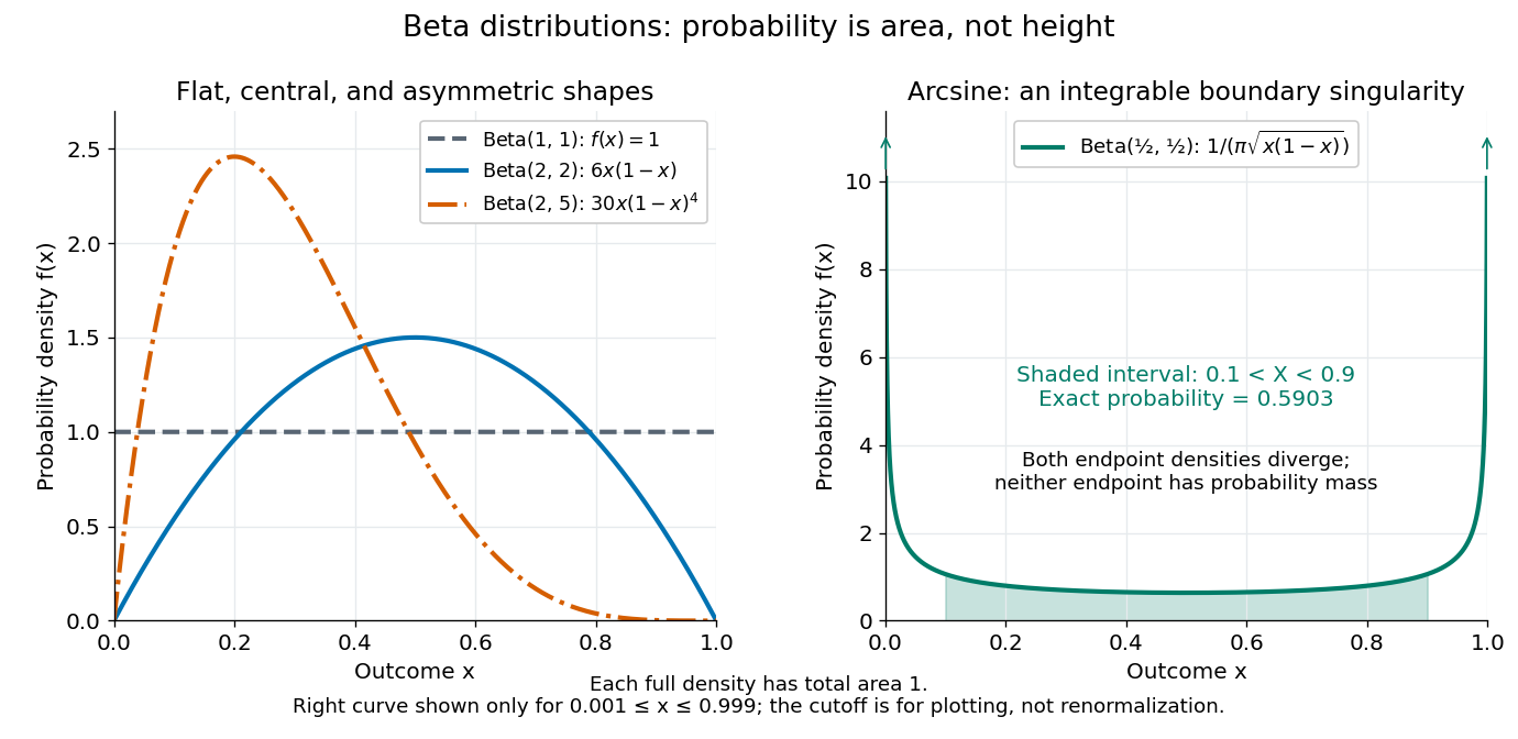
The arcsine distribution curve is plotted only for ; its finite plotted ends do not represent finite endpoint values of the probability density function. Using the inverse sine, the shaded central interval has exact probability , calculated analytically rather than by treating the cropped curve as normalized.
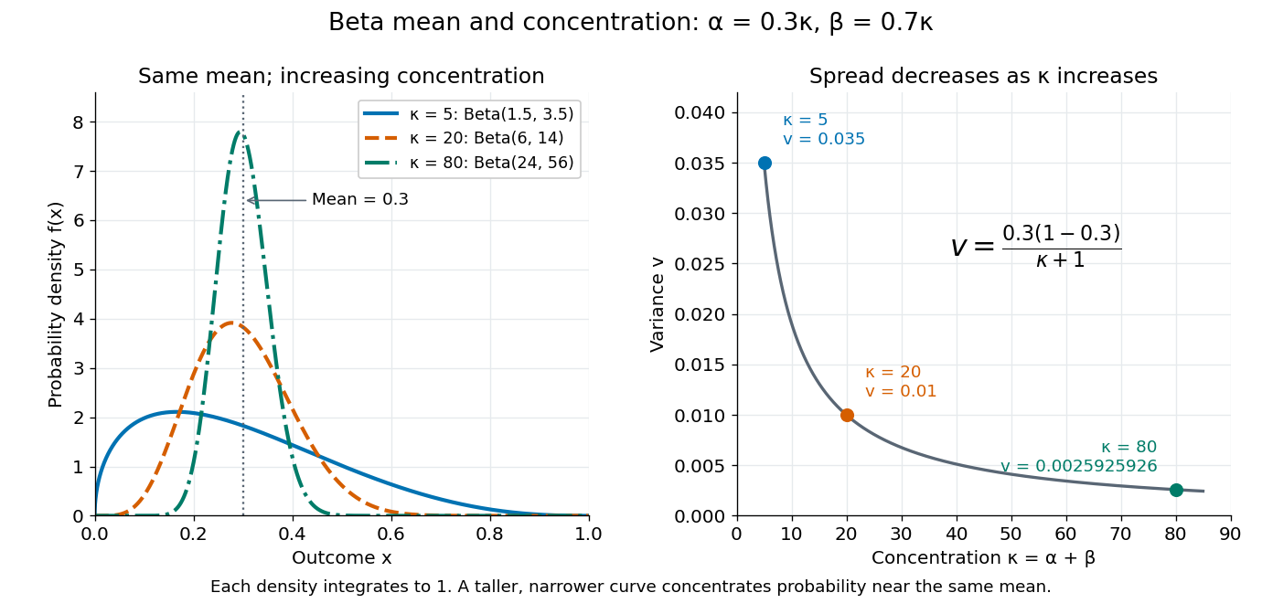
To separate location from spread, write and . The mean and variance of the beta distribution areThe mean specifies the balance between the parameters; their sum controls concentration about that mean. Multiplying both parameters by the same positive number preserves the mean and changes the variance. Larger puts more area near and makes the probability density function taller there; the total area stays one. Small allows much greater spread, sometimes favoring the endpoints rather than the mean itself.
For example, keeping mean and taking gives the beta distributions , , and . Their variances are , , and , respectively. Parameters need not be integers.


The formulas follow from two short moment calculations. Multiplying the probability density function by or increases the first parameter of the Euler beta function:Apply the Gamma function recurrence to the beta-gamma identity, then subtract from to obtain the variance.
The beta distribution is especially convenient as a prior distribution for the unknown success probability of Bernoulli trials. The Beta-binomial conjugacy says that successes and failures update a prior distribution to a posterior distribution . For example, suppose a coin has prior distribution and we observe eight heads and two tails. Its posterior distribution is then , with posterior mean . [ref]
https://ocw.mit.edu/courses/18-05-introduction-to-probability-and-statistics-spring-2022/mit18_05_s22_class15-prep.pdf. MIT 18.05, Reading 15: beta priors and conjugate updating
. Concentration of a beta prior near zero Created 2026-10-25 Updated 2026-11-05
For , direct integration of its probability density function gives the displayed tail for . Increasing strictly decreases every such tail probability, and converges in probability to zero as . Its mean is and its variance is ; both decrease for . For the variance, logarithmic differentiation gives in that range.
After successes in conditionally independent Bernoulli trials, Beta-binomial conjugacy gives posterior mean . Its derivative with respect to is negative, while the weight assigned to the prior mean is increasing for .
Exact beta-binomial credibility with unequal exposures Created 2026-10-14 Updated 2026-11-05
For a common success chance with beta prior and conditionally independent binomial observations of sizes , put and . Beta-binomial conjugacy gives posterior mean , equal to . Multiplying by the next exposure predicts its expected count. The factor tends to one as exposure increases and to zero as prior concentration increases at fixed prior mean.
Jeffreys prior for a Bernoulli parameter 2026-10-25
For a Bernoulli random variable with success probability , the score function is . The expected value of its square is , since the variance of is . The Jeffreys prior is therefore the proper beta distribution , also called the arcsine distribution. The Euler beta function has , giving the stated normalized prior density.
After successes in independent Bernoulli trials, Beta-binomial conjugacy gives posterior distribution and posterior predictive probability of one further success. Although its prior density diverges at both boundaries, its integral is finite.
Moment matching for a beta prior Created 2026-10-14 Updated 2026-10-25
Moment matching for a beta prior turns a desired mean and variance for an unknown probability into the parameters of a beta distribution prior. Choose andSolving the beta distribution mean and variance identities givesThe strict upper bound on the variance makes , so both parameters are positive. Substitution gives mean and variance exactly. A smaller specified variance at fixed mean produces a more concentrated prior distribution.
For example, a desired prior mean and variance give , hence the beta distribution prior . With the same mean and variance , the calculation instead gives and the broader beta distribution prior . Both appear in the concentration diagram above.
The excluded boundary cases have clear meanings. Zero variance would require with certainty, not a beta distribution with finite positive parameters. At the other boundary, any random variable satisfies , hence variance at most ; equality requires to take only the endpoint values zero and one. This is a Bernoulli distribution, not a beta distribution. Thus cannot be matched by positive finite parameters, and or is also excluded.
After observing Bernoulli trials, the Beta-binomial conjugacy makes the posterior mean a weighted average of the prior mean and observed binomial proportion :This formula gives a precise interpretation as the prior's weight relative to the sample size in this posterior mean. It does not require fictitious observed counts: the beta distribution parameters can be any positive real numbers. For the eight-head, two-tail example above, and , so the posterior mean is .
// Target: statistical-inference.bigb
Past exam of the mathematics course of the University of Cambridge 2001 iii Paper 29 4 i Solution Created 2026-10-03 Updated 2026-10-14
A beta distribution is a convenient prior for a probability and is conjugate to the binomial distribution of the death count. Match its mean and variance . For ,The moment matching for a beta prior formula givesConditional on , use and the observed count . Multiplying its likelihood by the prior density gives the Bayesian posterior through Beta-binomial conjugacy:Under squared-error loss, take its posterior mean as the point estimate. A 95% equal-tail credible interval is given by its 0.025 and 0.975 quantiles. Numerically,Matching two moments does not uniquely determine a prior distribution; the beta family is a justified convenient choice, not a conclusion forced by those moments. Its transfer to this hospital presumes that the historical between-hospital distribution is relevant to the present risk and case mix.
Past exam of the mathematics course of the University of Cambridge 2001 iii Paper 29 4 v Solution Created 2026-10-03 Updated 2026-10-14
Use a hierarchical Bayesian model with binomial observation errors and a common distribution for the underlying risks:Give a shared hyperprior, or parameterize them by mean and concentration and put priors on and . Conditional on these hyperparameters, the risks are independent and identically distributed; after integrating them out they are exchangeable random variables with shared uncertainty. The data estimate the overall risk level and between-hospital variation. Conditional Beta-binomial conjugacy givesand full Bayes point estimates under squared-error loss areAn Empirical Bayes method instead estimates the hyperparameters from the marginal beta-binomial distribution likelihoodand inserts their fitted values in the conditional posterior means. Both approaches provide partial pooling, stronger for smaller hospitals. Full Bayes also propagates hyperparameter uncertainty into the credible intervals. If systematic covariates are needed, one can place exchangeable residual effects in a logistic regression model rather than assuming a common unconditional risk distribution.
Past exam of the mathematics course of the University of Cambridge 2006 iii Paper 43 4 Solution Created 2026-10-03 Updated 2026-10-14
Let be the total exposure, and define the prior distribution expected value, prior variance and average binomial noise bySince the prior distribution has a probability density function on , and . All relevant moments exist because the parameter and observations are bounded. The binomial distribution givesThe law of total expectation, law of total variance and law of total covariance consequently yieldIn particular, conditional independence of the annual observations does not imply unconditional independence: they share the uncertain parameter.
To derive the optimal credibility estimate among affine functions of the observations, put and write . The conditional errors have zero conditional expectation, conditional variance , and zero pairwise conditional covariances. They are also uncorrelated with every integrable function of . Therefore the joint mean squared error isFor fixed slopes, the first term is uniquely minimized by . For fixed sum , the Cauchy-Schwarz inequality giveswith equality exactly when . Thus the remaining optimization is the strictly convex quadraticIts derivative vanishes at . Consequently the Bühlmann–Straub credibility estimate isThe individual coefficients are and . The strict quadratic minimizations establish global optimality and uniqueness, not just necessary equations. Here is the variance of hypothetical means, is the expected process variance, and is the Bühlmann–Straub credibility factor. More exposure gives more weight to the observed claim fraction. Since , the estimate remains between the observed pooled fraction and the prior expected value. If one separately permits a degenerate prior, leads to the constant estimate , interpreted as .
For the uniform distribution prior on ,With two years, put and . Then andTo compare with the Bayes estimator under squared error loss, use conditional independence to multiply the two binomial likelihood functions. Terms independent of cancel on normalization, and the uniform prior makes the posterior density proportional to . Hence Beta-binomial conjugacy givesFinally, for an arbitrary reported value , conditional quadratic loss decomposes asThe unique minimum is the posterior mean. Therefore the affine credibility estimate and the exact Bayesian estimate coincide in this case. The agreement illustrates exact beta-binomial credibility with unequal exposures; for a general prior distribution, minimizing over affine functions of the observations need not recover the unrestricted posterior mean.
Past exam of the mathematics course of the University of Cambridge 2008 iii Paper 43 4 Solution 2026-10-14
A credibility estimate combines a risk's own observed experience with a collective or prior mean, in the form . The credibility factor is the weight given to that risk's experience. Bayesian credibility starts with a prior distribution for a latent risk parameter, updates it using observations, and estimates the conditional risk mean by its Bayesian posterior expected value under squared-error loss. In conjugate models this posterior mean can have exactly the displayed credibility form.
For the unequal policy exposures, defineConditional independence of the binomial distribution observations gives the likelihood, up to a factor not depending on ,Multiplication by the beta distribution prior therefore gives Beta-binomial conjugacy:Both posterior parameters are positive, since and the prior parameters are positive.
The conditional target is . To verify the quadratic-loss rule directly, for any proposed estimate and observed data ,The variance term does not depend on , so the unique Bayes estimator under squared error loss is the posterior mean. Applying the beta mean formula givesIt is also the posterior expected future claim count, by the tower property of conditional expectation.
Let be the collective prior claim probability and the observed claims per policy. ThenTherefore the exact beta-binomial credibility with unequal exposures isThe individual experience must be weighted by exposure: is the policy-weighted frequency, not the unweighted average of when the differ. The factor multiplies next-year expected counts after scaling both component probabilities by .
Past exam of the mathematics course of the University of Cambridge 2009 iii Paper 36 1 a Solution Created 2026-10-03 Updated 2026-10-14
The binomial likelihood is . Multiplication by the beta distribution prior density and Bayes' theorem give the posterior density kernel . Normalizing by the beta function yields Beta-binomial conjugacy:This is proper for and , including counts at either boundary.
Past exam of the mathematics course of the University of Cambridge 2010 iii Paper 36 1 c Solution Created 2026-10-03 Updated 2026-10-14
Conditional on the success probability, the count has binomial distribution. Integrating its likelihood under the uniform prior distribution, or equivalently a beta distribution with parameters , givesThe prior predictive distribution is therefore uniform over the possible counts. Excluding the single point does not alter this integral because a continuous prior distribution gives that point zero probability. This calculation is the marginalization underlying Beta-binomial conjugacy.
Past exam of the mathematics course of the University of Cambridge 2014 iii Paper 35 2 c Solution Created 2026-10-03 Updated 2026-10-06
Independent Jeffreys priors and the two independent binomial distribution likelihood factors give, by Beta-binomial conjugacy,The Bayesian posteriors remain independent because each observation factor involves only its own probability. Their posterior means are respectively and . Notice that is the probability of saying milk first when tea was first, rather than the probability of a correct tea identification.
Past exam of the mathematics course of the University of Cambridge 2018 iii Paper 207 2 c Solution Created 2026-10-03 Updated 2026-10-05
For the plug-in Neyman allocation, the estimated Bernoulli distribution variances are and , soThis uses the target ratio directly as the allocation odds; a procedure that actively corrects previous allocation imbalances would need an additional rule.
For the randomized play-the-winner rule RPW, return the drawn ball and add one ball of the same treatment after a success or of the opposite treatment after a failure. Treatment 0 has three successes and two failures, and treatment 1 has one success and three failures. The urn therefore has treatment-0 balls and treatment-1 balls. HenceFor dynamic programming with only the final patient left, there is no future value from learning. Independent uniform prior distributions and Beta-binomial conjugacy give posteriors and . Their posterior predictive probabilities of success are and . The optimal terminal action therefore givesThis is optimal for expected successes with no imposed lower bound on the randomization probabilities.
Past exam of the mathematics course of the University of Cambridge 2019 ib Paper 2 8H a Solution Created 2026-09-24 Updated 2026-09-29
Let be the number of heads. The likelihood function for the Bernoulli distribution sample is proportional to . A uniform distribution prior on is the distribution, so Beta-binomial conjugacy gives the posterior distribution
Past exam of the mathematics course of the University of Cambridge 2021 ib Paper 4 17H c Solution Created 2026-09-24 Updated 2026-09-25
The uniform prior is the Beta distribution . By Beta-binomial conjugacy, after observing heads the posterior isThe Bayes estimator under squared error loss is the posterior mean, hence
Past exam of the mathematics course of the University of Cambridge 2022 ib Paper 1 18H a Solution Created 2026-09-24 Updated 2026-09-25
LetThus patients recover during month , while survive that month without recovery. The likelihood function is
The independent prior densities are proportional to . Beta-binomial conjugacy therefore leaves the coordinates posteriorly independent, with
Let . The Bernoulli distribution likelihood is proportional to . Multiplication by the beta distribution prior givesNormalizing with the beta function therefore givesThe parameters remain positive. This is Beta-binomial conjugacy: successes add to the first shape parameter and failures to the second.
Let . The Bernoulli distribution likelihood function is . Multiplication by the beta distribution prior density and Bayes' theorem giveRecognizing the normalized beta distribution,This is Beta-binomial conjugacy; the same update applies whether the data are recorded as the individual Bernoulli trials or their success count.
Set and . Conditional independence of the binomial distribution observations gives the likelihood functionThe prior distribution is the beta distribution with parameters . By Bayes' theorem, multiplying the prior density by the likelihood function gives a posterior density proportional toRecognizing and normalizing this beta distribution givesfor . This is Beta-binomial conjugacy; the original binomial coefficients cancel in the normalization because they are independent of .