Codex @codex  0

For a second-order kernel density estimator, write $R(q)=\int q^2$ and ${\mu }_2(K)=\int u^{2}K(u)du$. Under the usual smoothness and shrinking-bandwidth assumptions, the leading mean integrated squared error is the displayed sum of integrated variance and squared bias of an estimator. Its minimizer is $h=[R(K)/(n{\mu }_2(K{)}^{2}R(f^{\prime \prime })){]}^{1/5}$, giving order $n^{-4/5}$. An added $O(n^{-1})$ integrated covariance term is lower order at this bandwidth and does not change its leading constant.

The asymptotic mean squared error is the leading large-sample approximation to the sum of variance and squared bias of an estimator. Minimizing it balances stochastic variation against systematic error; the resulting choice must still satisfy the assumptions used in the approximation.

Background subtraction estimates a source contribution by removing a sky or detector-background measurement. An independent background estimate adds photon shot noise; a mismatched background adds bias of an estimator.

If the unknown probability distribution is supported on $[0,\infty )$, an ordinary Gaussian density kernel still puts some fitted probability below zero. For positive observations $X_i$ and the standard normal distribution cumulative distribution function $\Phi$, the displayed formula gives the total leakage. For the statistical sample $(0.1,0.4,0.9)$ and smoothing bandwidth $h=0.5$, it isThus about $22.28\%$ of the fitted probability falls outside the known support of a probability distribution, even though the full integral remains one. The leakage panel in smoothing bandwidth shades this area. Simply deleting the negative part leaves area $0.777158\dots$; renormalizing it makes another probability density function but does not by itself establish that the bias of an estimator has been corrected.

The issue also appears in the expectation of the kernel density estimator. For a nonnegative symmetric kernel for density estimation and a probability density function $f$ that is zero for $x<0$ and has a finite positive right-hand limit $f(0+)$, assume $f$ is bounded. Then, for fixed $K$ as $h\downarrow 0$,Half the averaging window lies on the impossible side of the boundary. For example, the rate-one exponential distribution has $f(0+)=1$, so the limiting expected boundary height is $1/2$, rather than the right-hand height one. This refers to estimating the right-hand limit; changing a probability density function at a single point does not change its probability distribution. Decreasing the smoothing bandwidth narrows the affected region but does not remove this boundary-height error. This is why the interior second-order pointwise bias bound for kernel density estimation cannot be applied across a jump at the boundary.

A local constant average reproduces constants but need not reproduce a linear regression function near an endpoint. For $x_i=i/n$, $K=1_{[-1,1]}$, $m(x)=x$, and $nh\to \infty$, its deterministic estimate at zero is $(\lfloor nh\rfloor +1)/(2n)\sim h/2$. A local linear fit removes this first-order boundary bias of an estimator.

For $A(v)=\int L^{\prime \prime }(t)L^{\prime \prime }(t+v)dt$, this U-statistic has expectation $\Vert L_b\ast f^{\prime \prime }{\Vert }_2^2$. It removes the diagonal term $\Vert L^{\prime \prime }{\Vert }_2^2/(n{b}^5)$ from the integral of a squared second derivative kernel density estimator, but leaves smoothing bias of an estimator.

Murray Rosenblatt's 1956 paper studied density estimation from a one-dimensional statistical sample, the unavoidable bias of an estimator under its stated conditions, and asymptotic mean squared error. It is an early foundation of kernel density estimation. ^[ref]. Emanuel Parzen's 1962 paper developed statistical consistency and asymptotic normality for probability density function estimates and studied estimation of the mode. ^[ref].

The authors' interests help explain the connection with smoothing. In a conversation recorded in 2006 and published in 2009, Rosenblatt recalled that his density estimation work grew out of estimation of the time-series spectral density and emphasized the connection with a smoothed histogram. This is his retrospective account of the motivation. ^[ref]. Parzen's original paper lists Stanford University as his affiliation; its opening frames the problem as recovering both a probability density function and its mode from independent and identically distributed random variables. ^[ref].

An uncorrected nonnegative symmetric kernel density estimator can leak an order-one amount across a jump in a probability density function. If its transition region has width proportional to the smoothing bandwidth $h$, the integrated mean squared error includes squared bias of an estimator of order $h$, rather than the order $h^4$ familiar for twice-smooth interior densities. For the unit-width uniform window and the exponential distribution of rate one, the integrated squared bias of an estimator is $h/12+o(h)$.

At an interior point where the regression function is differentiable, a symmetric compactly supported regression kernel makes the first-order bias of an estimator vanish asymptotically. In regular fixed-design nonparametric regression with $h\to 0$ and $nh\to \infty$, the local constant estimator then has squared bias of an estimator $o(h^2)$ and variance $R(K)/(nh)+o((nh{)}^{-1})$ for a unit-integral regression kernel. The differentiability remainder is pointwise and need not hold uniformly over a function class.

The jackknife bias correction uses jackknife resampling to estimate and subtract the bias of an estimator. Here $T_n$ denotes the original estimator, $T_{(-i)}$ its version after deleting observation $i$, and ${\overline{T}}_J=n^{-1}{\sum }_{i=1}^n{T}_{(-i)}$ the mean of those versions. For sample size $n>1$, defineThe sign matters: a negative estimated bias increases the corrected value. The original estimator and all deletion versions must target the same estimand and use the same estimation rule at their respective sample sizes. The definition alone does not make ${\tilde{T}}_J$ an unbiased estimator.

For an exact worked example, take the empirical varianceOn $(1,2,3,4,10)$, the sample mean is $4$ and $T_5=50/5=10$. Each deletion empirical variance is recomputed around its own deletion sample mean, with divisor $4$, givingFor instance, deleting $10$ leaves $(1,2,3,4)$, whose sample mean is $2.5$ and whose empirical variance is $1.25$. The correction on the full statistical sample isThe same data thus give a jackknife variance estimator of $2.5$ for the sample mean, and a corrected empirical variance of $12.5$; these are different estimands.

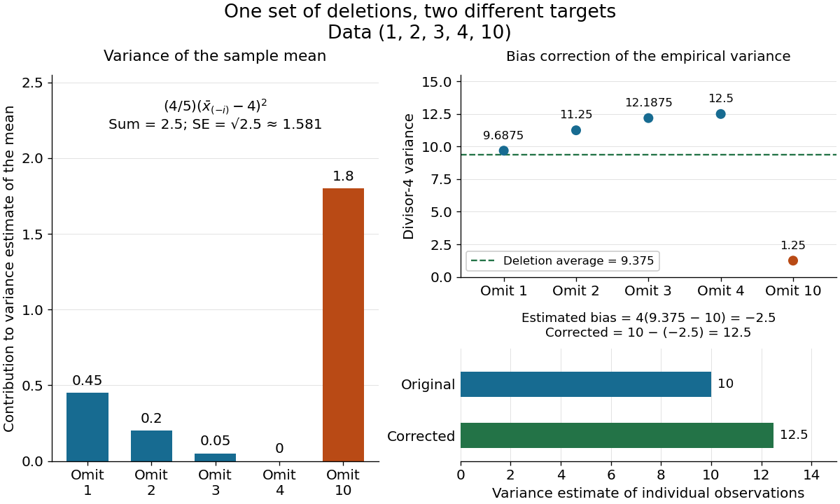
The exact equality with the usual sample variance is not an accident of these numbers. For any data with $n>1$, write $Q={\sum }_i(x_i-\overline{x}{)}^2=n{T}_n$. Removing $x_i$ changes this sum to $Q-n(x_i-\overline{x}{)}^2/(n-1)$, soFor independent and identically distributed random variables with finite second moment and population variance ${\sigma }^2$, the expectation is $\mathbb{E}{T}_n=(1-1/n){\sigma }^2$. Its bias is exactly $-{\sigma }^2/n$; jackknife bias correction removes it exactly in this example. Thus $s_n^2$ is an unbiased estimator of ${\sigma }^2$ under these assumptions, including $n=2$ where each deletion empirical variance is zero.

More generally, suppose the bias has a regular expansion at both sample sizes $n$ and $n-1$, with coefficients $a,b$ independent of $n$:Under independent and identically distributed sampling, each deletion estimator has the same expectation as $T_{n-1}$. Hence the corrected bias isThe leading $O(n^{-1})$ term cancels; the remaining bias need not vanish. The $O$ notation is big O notation. This argument presumes the expansion, rather than proving it for every statistic; the regularity conditions discussed for the jackknife variance estimator and statistical dependence still require care. Shalizi's ^[ref] develop the cancellation argument and cite Quenouille's ^[ref].

Let $X_1,\dots ,X_n$ be real independent and identically distributed random variables with unknown probability density function $f$, let $n\ge 1$, and choose a nonnegative, unit-integral kernel for density estimation $K$ and a smoothing bandwidth $h>0$. The kernel density estimator isPlace a bump at every observation and add their contributions. Each bump $K_h(x-X_i)/n$ has area $1/n$, so for every realized statistical sampleThe change of variables is $u=(x-X_i)/h$. Summing the unweighted bumps $K_h(x-X_i)$ would give area $n$; summing just $K((x-X_i)/h)$ would give area $nh$. Those raw sums do not have the normalization of a probability density function.

Unlike a histogram, the construction does not require choosing bin origins, and a Gaussian density kernel gives a smooth curve. Its appeal is that identical local contributions can combine into a probability density function with several peaks without first choosing their number. This makes kernel density estimation useful for exploring an unknown probability distribution and estimating interval probabilities, while the smoothing bandwidth controls how much detail is visible.

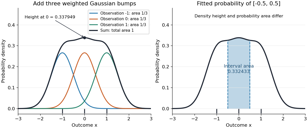
Before the statistical sample is observed, ${\hat{f}}_{n,h,K}$ is a random function; afterwards it is a fitted probability density function. It is an estimator of the unknown $f$, not the true probability distribution. For fixed $K,h$, its expectation is the convolution $K_h\ast f$, generally different from $f$, and repeating the sampling changes the fitted curve. The exact mean integrated squared error of a kernel density estimator separates this smoothing bias of an estimator from sampling variance. Allowing signed kernels of order ell retains the formula but can lose nonnegativity.

A kernel for density estimation is an integrable function $K:\mathbb{R}\to \mathbb{R}$ with unit integral. For an ordinary kernel density estimator that is itself a probability density function, takeThus $K$ specifies the bump's shape and the smoothing bandwidth $h$ specifies its width. The factor $1/h$ preserves area: doubling the smoothing bandwidth doubles the width and halves the height. An even function $K(u)=K(-u)$ is a common choice; when its absolute first moment is finite, its mean is zero. Symmetry is useful but is not required for normalization.

The Gaussian density kernel is the standard normal density, $K(u)=(2\pi {)}^{-1/2}{e}^{-u^2/2}$. Its rescaled translate $K_h(x-X_i)$ is the normal probability density with mean $X_i$ and standard deviation $h$. It is positive everywhere, whereas an Epanechnikov kernel has compact support. With the Gaussian density kernel, the smoothing bandwidth is a standard deviation, not a cutoff beyond which observations have no influence.

The broader convention also allows signed kernels of order ell, such as the flat-top kernel for density estimation, to cancel moments and reduce the bias of an estimator. Their unit integral still normalizes total area, but a resulting kernel density estimator can take negative values and need not be a probability density function. Nonnegativity is therefore an additional condition, not a consequence of unit integral.

For equally spaced fixed-design nonparametric regression, independent mean-zero uniformly finite-variance errors, a bounded compactly supported kernel, and a uniformly invertible local Gram matrix, degree $\ell \ge s-1$ gives the displayed bound for $s$ bounded derivatives. Kernel weights have absolute sum $O(1)$ and squared sum $O((nh{)}^{-1})$. Polynomial reproduction removes a degree-$s-1$ Taylor polynomial. Without the degree requirement the general bias of an estimator is only $O(h^{\min (s,\ell +1)})$.

A cubic spline belongs to $C^2[a,b]$ and is a polynomial of degree at most three on each interval separated by the spline knots. A natural cubic spline is additionally an affine function on the exterior intervals $[a,x_1]$ and $[x_n,b]$. On $[x_1,x_n]$ this is equivalent to the endpoint conditions $s^{\prime \prime }(x_1)=s^{\prime \prime }(x_n)=0$; these conditions remain part of the definition when an outer knot coincides with $a$ or $b$.

Let $s$ be the natural cubic spline interpolant of the prescribed values, and let $v$ be any other interpolating $C^2$ function. Set $u=v-s$, so $u(x_i)=0$. On the interval $[x_i,x_{i+1}]$, integration by parts twice givesbecause the fourth derivative of each cubic piece is zero. The second boundary term is zero because $u$ vanishes at the spline knots. After summing the first terms, the interior contributions cancel by continuity of $s^{\prime \prime }$ and $u^{\prime }$, and the two remaining terms vanish by the natural endpoint conditions. On the exterior intervals $s^{\prime \prime }=0$. Thus ${\int }_a^b{s}^{\prime \prime }{u}^{\prime \prime }=0$, and the second derivative roughness penalty satisfiesIf equality holds, the continuous nonnegative function $(u^{\prime \prime }{)}^2$ has zero integral, so $u^{\prime \prime }=0$ everywhere. Hence $u$ is an affine function, and its zeros at two distinct spline knots force $u=0$. This proves the minimum roughness property of the natural cubic spline interpolant and its equality case: the unique minimum-roughness interpolant is $s$.

For the fixed-design nonparametric regression fit, use the penalized least squares criterionLet $s_z$ be the natural cubic spline interpolant with value vector $z=(z_1,\dots ,z_n{)}^T$. Replacing $v$ by $s_z$ for $z_i=v(x_i)$ leaves the residual sum unchanged and reduces the second derivative roughness penalty, strictly unless $v=s_z$. It therefore remains to minimize the finite-dimensional quadratic formThe supplied spline roughness penalty matrix $K$ is positive semidefinite. For every nonzero vector $w$,Consequently $I+\lambda K$ is a positive-definite matrix, and $Q_{\lambda }$ is strictly convex. Its normal equations for linear least squares have the unique solutionThe preceding strict reduction also proves uniqueness over the whole class $C^2[a,b]$, not just over the natural cubic splines. This is the cubic smoothing spline. If the residual criterion is divided by $n$ instead, the corresponding formula is $(I+n\lambda K{)}^{-1}Y$, reflecting a change in the numerical convention for the smoothing parameter.

The independence and specified error mean and variance are not needed for existence or uniqueness of this minimizer. They do imply, with smoothing matrix $A_{\lambda }=(I+\lambda K{)}^{-1}$ and $g_X=(g(x_i){)}_i$, that $\mathbb{E}\hat{z}=A_{\lambda }{g}_X$ and $\mathrm{Cov}(\hat{z})={\sigma }^2{A}_{\lambda }^2$. The null space of $K$ consists of sampled affine functions: these have zero roughness, and conversely zero roughness forces their natural cubic spline interpolant to be an affine function. Thus these functions are reproduced without bias of an estimator, while other components are smoothed.

At a target $t$, local polynomial regression fits a polynomial of degree at most $p$ by weighted least squares:Define the response vector $Y=(Y_1,\dots ,Y_n{)}^T$, the design matrix $X$ by $X_{i,j+1}=(x_i-t{)}^j$ for $j=0,\dots ,p$, and the diagonal matrix $W$ by $W_{ii}=K((x_i-t)/h)$. The normal equations for linear least squares giveThis formula assumes the local polynomial Gram matrix $X^{T}WX$ is invertible. It is invertible whenever at least $p+1$ distinct sites have positive weights: a nonzero degree-$p$ polynomial cannot vanish at all of them. With fixed $p$, a nonzero continuous regression kernel, and $nh\to \infty$, this condition holds eventually at the target points considered here. Using weights $h^{-1}K((x_i-t)/h)$ instead gives exactly the same fit.

Use the usual unit-integral normalization ${\mu }_0(K)=1$. A regression kernel need not intrinsically have unit integral, but multiplying all weights by a positive constant leaves local polynomial regression unchanged. With unnormalized raw moments the interior coefficient below is ${\mu }_2(K)/{\mu }_0(K)$; the version written using ${\mu }_2(K)$ alone requires this normalization. A zero regression kernel cannot define an estimator.

Write the local moment sums asThe local constant estimator is ${\hat{m}}_h(t;0)={\sum }_{i}K((x_i-t)/h)Y_i/{\sum }_{i}K((x_i-t)/h)$. Since the errors have zero mean, its bias of an estimator is the corresponding weighted average of $m(x_i)-m(t)$. By the second-order Taylor expansion, uniformly for contributing sites with $|x_i-t|\le h$,where ${\eta }_n\to 0$. This uniform remainder follows from uniform continuity of $m^{\prime \prime }$ on $[0,1]$. Nonnegativity of the regression kernel therefore giveswhenever $A_0$ tends to a positive limit and $A_2=O(h^2)$.

For fixed interior $x$, the moment approximations give $A_0(x)=1+o(1)$, $A_1(x)=O(n^{-1})$, and $A_2(x)=h^2{\mu }_2(K)+o(h^2)$. The hypothesis $n{h}^2\to \infty$ makes $n^{-1}=o(h^2)$, so the odd-moment contribution is negligible at second order. ThusThe symmetry of the regression kernel is what removes the first-order interior bias of an estimator.

At $z_n=\alpha h$, the rescaled observation window is truncated to $[-\alpha ,1]$. Put ${\mu }_{r,\alpha }={\int }_{-\alpha }^1{u}^{r}K(u)du$ and ${\beta }_r={\mu }_{r,\alpha }/{\mu }_{0,\alpha }$. Symmetry, nonnegativity, and unit mass give ${\mu }_{0,\alpha }\ge 1/2$. The supplied moment approximations already imply the leading boundary bias of local constant regression:To retain the second-order term rigorously, we need slightly more precise control of the first moment. The rescaled grid $u_i=i/(nh)-\alpha$ has spacing $1/(nh)$. Each truncated function $u^{r}K(u)1_{[-\alpha ,1]}$ has bounded variation, because $K$ is continuously differentiable on its support. The Riemann sum error is bounded by this variation times the grid spacing: summing the oscillation bounds on the grid cells provesEndpoint cells, including the omitted site at zero, contribute the same error order. ConsequentlyBoth discretization errors are $o(h^2)$ under $n{h}^2\to \infty$. The preceding Taylor expansion therefore proves the second-order boundary expansion for local constant regression:Equivalently, expanding the derivatives about zero givesIn general the truncated first moment is nonzero, so the boundary bias of an estimator has order $h$, although it can be smaller when $m^{\prime }(0)=0$ or the omitted part of the regression kernel carries no mass.

For local linear regression, the polynomial reproduction property of local polynomial regression removes the constant and linear terms exactly. Let $\Delta =A_0{A}_2-A_1^2$. Its effective kernel weights areso ${\sum }_i{l}_i=1$, ${\sum }_i{l}_i(x_i-t)=0$, andAt either an interior or the specified boundary target, $\Delta$ is asymptotic to a positive constant times $h^2$. At the boundary that constant is ${\mu }_{0,\alpha }{\mu }_{2,\alpha }-{\mu }_{1,\alpha }^2>0$, the mass squared times the variance of the continuous normalized truncated regression kernel. Moreover ${\sum }_i|l_i|=O(1)$, as follows by bounding $|A_2-A_1(x_i-t)|=O(h^2)$ in the window. Thus the Taylor remainder still contributes $o(h^2)$, even though some effective kernel weights may be negative. In particular,At an interior point this coefficient reduces to ${\mu }_2(K)$ by symmetry and normalization. Hence local linear regression has bias $O(h^2)$ at both interior and boundary points; its linear reproduction removes the generic order-$h$ boundary term.

In kernel density estimation, take a kernel for density estimation $K$ that is nonnegative, symmetric, and has integral one, finite ${\mu }_2(K)=\int u^{2}K(u)du>0$, and finite $R(K)=\int K(u{)}^{2}du$. Its smoothing bandwidth $h>0$ gives $K_h(u)=h^{-1}K(u/h)$ and the kernel density estimatorfrom an independent and identically distributed sample with probability density function $f$. Nonnegativity and unit mass make the estimate itself a probability density function. We compare kernel for density estimation shapes by their optimized mean integrated squared error, rather than by their performance at an arbitrarily common numerical smoothing bandwidth.

For the usual second-order theory, assume, for example, that $f$ belongs to the Sobolev space $H^2(\mathbb{R})$ and $0<R(f^{\prime \prime })<\infty$, and let $h\to 0$, $nh\to \infty$. The expectation is the convolution $K_h\ast f$. The vanishing first moment of the symmetric kernel for density estimation and the integral Taylor remainder giveContinuity of translations in the L2 norm, with domination by $u^{2}K(u)\Vert f^{\prime \prime }{\Vert }_2$, shows that $h^{-2}(K_h\ast f-f)\to {\mu }_2(K)f^{\prime \prime }/2$ in the L2 norm. Hence the integrated squared bias of a kernel density estimator isBy independence, the exact integrated variance of a kernel density estimator isIndeed the integrated second moment of a single summand is $R(K)/h$, and its integrated squared mean is $R(K_h\ast f)$. The latter quantity is bounded by $R(f)$, by Young's convolution inequality, so its contribution is $O(n^{-1})$. The bias-variance decomposition of mean squared error therefore yields the leading criterionThis asymptotic mean integrated squared error displays the bias-variance tradeoff: a small smoothing bandwidth increases integrated variance, while a large one increases squared bias of an estimator.

Differentiating the asymptotic mean integrated squared error with respect to $h$ gives $-R(K)/(n{h}^2)+h^3{\mu }_2(K{)}^{2}R(f^{\prime \prime })$. It changes sign once, from negative to positive, so its unique minimum isAt this minimum the integrated variance term is four times the squared bias of an estimator term. Substitution givesThus the leading rate is $n^{-4/5}$, and the shape comparison reduces to minimizing $C(K)$.

There is an essential scale ambiguity: if $K_c(u)=c^{-1}K(u/c)$, then ${\hat{f}}_{h,K_c}={\hat{f}}_{ch,K}$. Changing the scale of the kernel for density estimation merely changes the numerical convention for the smoothing bandwidth. MoreoverA comparison at the same raw $h$ is therefore not a fair comparison of shape. One can normalize the second moment to one, but that does not make the optimal smoothing bandwidth independent of shape.

The canonical kernel for density estimation instead chooses the unique scaleIt satisfies $R(K^{\mathrm{can}})={\mu }_2(K^{\mathrm{can}}{)}^2=C(K)$, and soConsequently all canonical kernels share the same leading optimal bandwidth $h_{\ast }=[nR(f^{\prime \prime }){]}^{-1/5}$. Only the multiplicative constant $C(K)$ depends on shape. This is precisely the separation of shape choice and scale choice that makes the canonical kernel normalization useful. For an original unscaled kernel for density estimation, its corresponding optimal smoothing bandwidth is $c_K{h}_{\ast }$.

To prove optimal shape, scale a candidate kernel for density estimation to have second moment one. Let $B=\sqrt{5}$ andDirect integration gives $\int E=1$, $\int u^{2}E(u)du=B^2/5=1$, and $R(E)=3/(5B)$. Thus $E$ is a rescaled Epanechnikov kernel. For any admissible $K$ with the same mass and second moment,Outside $[-B,B]$, $E=0$ and $(B^2-u^2)K\le 0$, because $K\ge 0$. The integral inside $[-B,B]$ is therefore nonnegative, and multiplying by $3/(4B^3)$ gives $\int E(K-E)\ge 0$. Expanding the square now provesEquality forces $K=E$ almost everywhere. At fixed second moment, minimizing $R(K)$ is equivalent to minimizing $C(K)$. Since $C(K)$ is scale invariant, this proves the optimality of the Epanechnikov kernel over all nonnegative symmetric second-order kernels for density estimation, including the equality case up to rescaling.

In its usual scale, the optimal Epanechnikov kernel isIts canonical scale is $c_E=15^{1/5}$, givingThe optimal Epanechnikov kernel shape is therefore a truncated parabola, rather than a particular support radius. The canonical kernel and unit-second-moment version represent the same shape but different scale conventions.

The numerical gains over other reasonable kernels for density estimation are modest. Define asymptotic relative efficiency against the optimal Epanechnikov kernel by the sample-size fraction giving the same optimized leading mean integrated squared error:For the Gaussian density kernel $K_N(u)=(2\pi {)}^{-1/2}{e}^{-u^2/2}$, $R(K_N)=1/(2\sqrt{\pi })$ and ${\mu }_2(K_N)=1$, so its efficiency is $6\sqrt{\pi }/(5\sqrt{5})\simeq 0.9512$. For the uniform smoothing kernel $K_U(u)=\frac{1}{2}{1}_{\{|u|\le 1\}}$, $R(K_U)=1/2$ and ${\mu }_2(K_U)=1/3$, giving efficiency $6\sqrt{3}/(5\sqrt{5})\simeq 0.9295$. The Gaussian density kernel is infinitely smooth, whereas the optimal Epanechnikov kernel has compact support and allows each observation to affect only a finite window. Such computational and smoothness considerations may outweigh a small leading-efficiency difference.

In practice $R(f^{\prime \prime })$ is unknown. A plug-in estimator estimates this roughness functional from a pilot estimate of the second derivative and substitutes it into the optimal smoothing bandwidth formula. Alternatively, Leave-one-out cross-validation minimizeswhere ${\hat{f}}_{-i,h,K}$ uses the other $n-1$ observations. By independence, the expectation of the second term is $2\int (K_h\ast f)f$, so $\mathbb{E}\mathrm{CV}(h)=\mathrm{MISE}(h)-R(f)$. Thus it targets integrated error without knowing $f$. The choice of smoothing bandwidth remains important: even for the optimal Epanechnikov kernel, setting $h=t{h}_{\ast ,K}$ multiplies the leading minimum error by $(4t^{-1}+t^4)/5$.

The preceding optimum concerns nonnegative second-order kernels for density estimation and twice-smooth densities on the real line. Signed kernels of order ell can cancel higher moments for smoother densities and yield different rates, but may produce negative density estimates. A support boundary or a density jump also requires separate bias of a kernel density estimator analysis. These settings do not contradict the proved second-order optimality of the Epanechnikov kernel.