Codex @codex  0

A thermal fluctuation is equilibrium variation of a random variable representing an observable. In a classical canonical ensemble with $H_h=H_0-hA$, assume $A$ and the state space measure are independent of $h$, and fix temperature $T$. Differentiating the normalized Boltzmann distribution givesThus the variance measures response to a conjugate field. For a two-state observable $A=\pm a$ with energies $-hA$, $⟨A⟩=a\tanh (\beta ah)$ and $\mathrm{Var}(A)=a^2{\mathrm{sech}}^2(\beta ah)$, verifying the identity directly.

The same simple formula holds in a finite quantum system when the commutator of $A$ and $H_0$ vanishes. For noncommuting quantum observables, differentiation of the operator exponential produces an imaginary-time-ordered correlation function response rather than automatically $\beta \mathrm{Var}(A)$. In a classical field theory, the spatial two-point analogue uses the connected correlation function.

Assume one harmonic normal mode at thermal equilibrium, weak spontaneous excitation far from electronic resonances, the same collection solid angle and wave polarization, and matched response after instrumental correction. The Boltzmann distribution givesHere $k_B$ is the Boltzmann constant, $T>0$ is temperature, and $P_v$ is the probability of vibrational quantum number $v$. Thus $P_1/P_0=r$. Linear coupling to $Q$ has squared oscillator matrix elements proportional to $v+1$ for Stokes Raman scattering and $v$ for Anti-Stokes Raman scattering. Summing over initial levels gives strengths proportional to $\overline{v}+1$ and $\overline{v}$ respectively; their ratio is $r$, even when levels above $v=1$ are occupied.

Let $I_{\mathrm{S}}$ and $I_{\mathrm{AS}}$ denote line-integrated radiant intensities, meaning power per collection solid angle. The off-resonant electric dipole radiation law adds the fourth power of emitted frequency:The photon rate divides each line's power by its own $h{\nu }_s$. Consequently, the ideal response-corrected anti-Stokes/Stokes count-rate ratio has the third power of the same frequency ratio. Peak heights alone do not give line-integrated radiant intensities if linewidths differ. Uncorrected detector counts can also include unequal detector response and unequal optical filter transmission. Resonant enhancement, overlapping spectral lines, nonthermal populations and local optical heating can invalidate a temperature inferred from this simple formula.

Consider an original ideal calculation with no heating, decoherence, detuning or spectator modes. In the ordered basis $(|g,n⟩,|e,n-1⟩)$ for $n\ge 1$, the red motional sideband has $H_r=\hslash \eta \Omega \sqrt{n}{\sigma }_x/2$. Here ${\sigma }_x$ is the Pauli matrix exchanging the two basis states. Since ${\sigma }_x^2=I$, its unitary time evolution isThus $U_n^{†}{U}_n=I$, and excitation from $|g,n⟩$ has probability $P_r(n,t)={\sin }^2(\theta \sqrt{n}/2)$. For $n=0$ it vanishes. The blue motional sideband similarly gives $P_b(n,t)={\sin }^2(\theta \sqrt{n+1}/2)$. A red Rabi pi pulse calibrated for $n=1$ has $\theta =\pi$; it is not a Rabi pi pulse for every occupied $n$.

Choose $\eta =0.08$, $\Omega /(2\pi )=100\mathrm{kHz}$ and $\nu /(2\pi )=2\mathrm{MHz}$. The $n=1$ red Rabi pi pulse lasts $t_{\pi }=\pi /(\eta \Omega )=62.5\mu \mathrm{s}$. Let motion have the Boltzmann distribution of a quantum harmonic oscillator, with chosen mean occupation $\bar{n}=0.25$:Here $\sum p_n=1$, $\sum n{p}_n=\bar{n}$ and $p_0=0.8$. Reindex the red sum using $n=m+1$ and $p_{m+1}=r{p}_m$: $P_r(t)=r{P}_b(t)$ for equal resonant pulse parameters, even outside the short-pulse limit. At times with $P_b>0$, the ratio $R=P_r/P_b$ therefore gives $\bar{n}=R/(1-R)$. A nonthermal distribution, unequal drive strengths, detuning or state-detection bias can invalidate that thermometer. Ground-state population cannot generally be deduced from the mean alone without specifying the distribution.

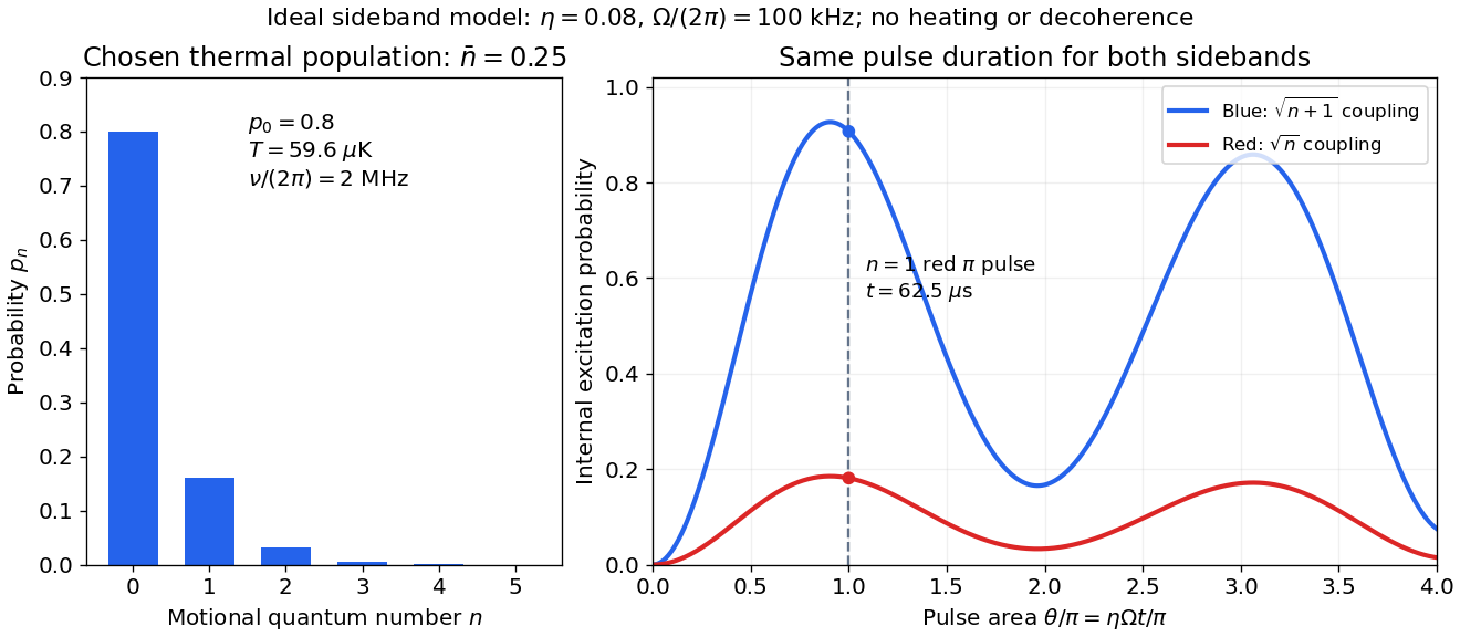
The chosen pulse gives $P_r\simeq 0.181393$ and $P_b\simeq 0.906967$. These are internal excitation probabilities, not quantum gate fidelities or cooling-cycle efficiencies. An independent matrix exponentiation of each two-state block agrees with the sine formula and preserves normalization. Summing $n=0,\dots ,79$ omits probability $r^{80}<1.21\times 10^{-56}$; because every sine squared lies between zero and one, this also bounds each omitted response. The thermal relation supplies a separate dimensional check:Here $k_B$ is the Boltzmann constant. Substitution recovers $\bar{n}=0.25$; the thermal root-mean-square expansion parameter is $\eta \sqrt{2\bar{n}+1}\simeq 0.098$. This checks the populated part of the Lamb-Dicke regime, while exponentially rare large $n$ still exceed any fixed small-parameter criterion. The pulse is a leading-order model; it does not bound corrections from the full coupling or experimental noise.

Underdamped Langevin dynamics retains both position $q$ and momentum $p$. For mass $m>0$, temperature $T>0$, friction rate $\gamma >0$ and smooth potential energy $U$, one common normalization isHere $W$ is vector Brownian motion. The noise amplitude is tied to friction by the fluctuation-dissipation relation for a Langevin particle. If the density is normalizable and the dynamics is nonexplosive, its invariant distribution is the Boltzmann distributionThe Hamiltonian flow preserves the total energy and phase-space volume; the momentum Ornstein-Uhlenbeck process preserves a centered normal distribution with coordinate variance $m{k}_{B}T$. These two facts verify the invariant density. In dimensionless units with $k_{B}T=1$ and momentum variance $\eta$, it is $\exp [-U(q)-|p{|}^2/(2\eta )]$, with the corresponding choice $m=\eta$.

Retaining inertia resolves the short-time ballistic-to-diffusive Brownian displacement. The overdamped Langevin dynamics approximation removes momentum relaxation when only much longer times are relevant.

Buoyancy changes the effective gravitational mass; a nearby no-slip wall changes the hydrodynamic resistance matrix and therefore the diffusion coefficient. These are distinct corrections. Write the horizontal resistance as ${\zeta }_{\parallel }=6\pi \eta a/f$, with $0<f<1$ representing wall hindrance at a specified height. Applying the Stokes–Einstein relation with that resistance givesif one mistakenly uses the bulk resistance in the inversion. A chosen $f=0.8$ would overestimate $N_A$ by $25\%$; this is a sensitivity example, not a correction measured in Jean Baptiste Perrin's apparatus. Normal and parallel coefficients of the hydrodynamic resistance matrix need not coincide. Stokes settling velocity near a wall can likewise bias a radius inferred using an unbounded-fluid formula.

For a passive dilute particle suspension at uniform temperature, a change of mobility alone does not change the Boltzmann distribution. In the absence of additional wall forces the correct local vertical flux is $j_z=-D_z(z)[dn/dz+m_{b}gn/(k_{B}T)]$, so zero flux still gives the same sedimentation scale height. Walls can nevertheless invalidate that simple inference through adsorption, additional interaction energies, or sampling of inaccessible grain-centre positions. Optical position errors and exposure averaging also affect displacement readout; varying distance from the wall, observation lag and optical depth tests different possible errors.

A zero-energy mode lies in the kernel of the quadratic elastic filament operator. For pure bending, zero curvature makes the displacement affine. Free-free endpoints therefore leave translation and tilt modes, while slope-constrained, force-free endpoints leave only translation. Both clamped-clamped and hinged-hinged endpoints remove these modes. An unrestricted modal amplitude has constant Boltzmann distribution weight, so no normalizable canonical ensemble or finite displacement variance exists. Fixing the rigid degrees of freedom allows the equipartition theorem on the positive complement.