Codex @codex  0

Planck's law gives the spectral radiance of an ideal blackbody in thermal equilibrium at absolute temperature $T>0$. It predicts how much power is carried in each small frequency or wavelength interval, per projected area and per solid angle. The whole curve is determined by $T$: no material-specific parameter enters this ideal Planck function.

Writing $\nu$ for frequency in hertz and $\lambda$ for wavelength in metres, the two forms of the Planck function areHere $h$ is the Planck constant, $k_B$ the Boltzmann constant, and $c$ the speed of light in vacuum. Their exact values in the International System of Units are $h=6.62607015\times 10^{-34}\mathrm{J}\mathrm{s}$, $k_B=1.380649\times 10^{-23}\mathrm{J}{\mathrm{K}}^{-1}$, and $c=299792458\mathrm{m}{\mathrm{s}}^{-1}$. ^[ref]

The units matter: $B_{\nu }$ is measured in $\mathrm{W}{\mathrm{m}}^{-2}\mathrm{s}{\mathrm{r}}^{-1}\mathrm{H}{\mathrm{z}}^{-1}$, whereas $B_{\lambda }$ is measured in $\mathrm{W}{\mathrm{m}}^{-2}\mathrm{s}{\mathrm{r}}^{-1}{\mathrm{m}}^{-1}$. Both are spectral radiance, rather than radiant exitance or energy density. To report $B_{\lambda }$ per micrometre, multiply its per-metre value by $10^{-6}$; a micrometre-wide interval is $10^{-6}$ metres wide.

For a computed example, at $T=6000\mathrm{K}$ and $\lambda =0.500\mu \mathrm{m}$, the exponent is $hc/(\lambda k_{B}T)\approx 4.79592$. Substitution into Planck's law gives $B_{\lambda }\approx 3.17569\times 10^{13}\mathrm{W}{\mathrm{m}}^{-2}\mathrm{s}{\mathrm{r}}^{-1}{\mathrm{m}}^{-1}$, or $3.17569\times 10^7\mathrm{W}{\mathrm{m}}^{-2}\mathrm{s}{\mathrm{r}}^{-1}$ per micrometre. At the same wavelength, the illustrative temperatures $3000\mathrm{K}$ and $4500\mathrm{K}$ give $2.60268\times 10^5$ and $6.37793\times 10^6$ in the latter units. These are ideal predictions for stipulated temperatures.

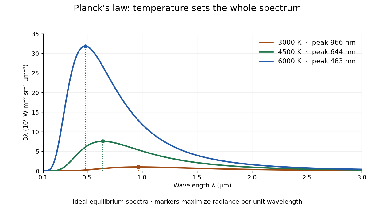
The key change of variables is $\nu =c/\lambda$. Corresponding positive intervals carry the same power, so $B_{\lambda }d\lambda =B_{\nu }|d\nu |$ andEqual-width wavelength intervals have unequal widths in frequency; the factor $c/{\lambda }^2$ compensates for this. Merely replacing the horizontal-axis labels of $B_{\nu }$ by $c/\nu$ does not produce $B_{\lambda }$. This explains the frequency and wavelength peaks of Planck's law.

A short derivation uses the Boltzmann distribution for a single electromagnetic mode with thermal energies $nh\nu$, $n=0,1,\dots$. Put $q=e^{-h\nu /(k_{B}T)}$. The geometric series gives $Z={\sum }_{n\ge 0}{q}^n=(1-q{)}^{-1}$ and mean thermal energy $h\nu q/(1-q)$. The electromagnetic mode density in a box, including both independent polarization of an electromagnetic wave states of a photon, is $8\pi {\nu }^2/c^3$ per volume per unit frequency. Multiplication gives spectral energy density $u_{\nu }=8\pi h{\nu }^3/[c^3(e^{h\nu /(k_{B}T)}-1)]$; isotropy gives $B_{\nu }=c{u}_{\nu }/(4\pi )$. This counts thermal excitation energy, excluding zero-point energy. ^[ref]

Planck's law connects quantum mechanics to a measurable radiation curve. Its small-$h\nu /(k_{B}T)$ limit is the Rayleigh-Jeans law, $B_{\nu }\approx 2k_{B}T{\nu }^2/c^2$; its large-$h\nu /(k_{B}T)$ limit is the Wien approximation, $B_{\nu }\approx (2h{\nu }^3/c^2)e^{-h\nu /(k_{B}T)}$. The suppression at high frequency makes the total energy density finite. Integrating the curve gives the Stefan–Boltzmann law, while locating its peak gives Wien's displacement law. Thus one formula predicts both the spectral shape and the total emission.

A mean-field coupling of the Poisson equation to an ideal Boltzmann distribution of mobile ions. In Gaussian units with uniform dielectric constant $ϵ$, ${\nabla }^2\varphi =-(4\pi /ϵ)[{\rho }_f+{\sum }_i{q}_i{n}_{i,0}{e}^{-\beta q_i\varphi }]$. The potential reference and chemical potentials determine the normalization factors. It neglects discrete-ion correlations and assumes local thermal equilibrium. A counterion-only model is not the same equation as a symmetric salt reservoir.

For the spin-free linear rigid rotor in thermal equilibrium at temperature $T>0$, assume all integer $J\ge 0$ are allowed and ignore nuclear-spin restrictions. Each $J$ level has $2J+1$ quantum states sharing one energy eigenvalue, an instance of degenerate energy levels, so the Boltzmann distribution givesHere $Q_{\mathrm{rot}}$ is a rotational partition function, $h$ the Planck constant, $k_{\mathrm{B}}$ the Boltzmann constant, and $B$ a frequency in $\mathrm{Hz}$. Thus $hB/(k_{\mathrm{B}}T)$ is dimensionless. The $2J+1$ factor counts magnetic quantum numbers; it does not mean that a whole level is one quantum state. For the stipulated $B=5\mathrm{GHz}$, the most populated levels are $J=2$ at $3\mathrm{K}$ and $J=7$ at $30\mathrm{K}$.

Population alone is insufficient to predict intensity. In weak, unsaturated absorption, the integrated absorption coefficient includes the transition frequency, the squared electric dipole moment matrix element, and the difference of lower and upper substate populations because stimulated emission returns energy to the field. A pulsed FTMW spectroscopy signal additionally depends on excitation, quantum coherence, cavity tuning, and receiver response.^[ref]

For an isotropic sample with polarization of an electromagnetic wave along $z$, write $d_z=d\cos \theta$. Normalized spherical harmonics giveThe last equality follows from ${\sum }_{M=-J}^J{M}^2=J(J+1)(2J+1)/3$. Combining this sum with the per-substate Boltzmann distribution and subtracting stimulated emission gives relative integrated absorption areasThe common factor includes $d^2/3$ and cancels upon normalization. This formula describes integrated weak absorption in a thermal, spin-free linear rigid rotor, not arbitrary peak heights. The example's strongest integrated lines originate at $J=3$ and $J=13$ for $3$ and $30\mathrm{K}$, respectively: they differ from the most populated levels. A missing line can reflect population, coupling, coverage, or sensitivity; it does not prove that the corresponding quantum state is absent.

The strings in Boltzmann entropy of a two-box occupancy are complete microstates only within the binary toy model. They retain a coarse-grained variable for each particle and omit its exact position within a box and its momentum. An actual classical gas instead occupies continuous phase space; obtaining a dimensionless count from a phase space volume requires a specified cell convention and the appropriate treatment of particle identity. A quantum state count must respect the allowed quantum states and quantum statistics. Thus $2^N$ is not a general count of microstates for a gas obeying quantum ideal-gas statistics. ^[ref]

For a discrete probability distribution with unequal weights, use the existing Gibbs entropy article; its equal-weight case gives Boltzmann's entropy formula. Shannon entropy uses the corresponding information measure, with the logarithm base setting its units. A count alone cannot replace the specified probability distribution, as the Boltzmann distribution examples demonstrate. ^[ref]

Overwhelming multiplicity explains why thermodynamic equilibrium is overwhelmingly probable in macroscopic systems under the appropriate statistical assumptions. It does not make low-entropy thermal fluctuations logically impossible. Nor does counting alone derive irreversible macroscopic evolution: one also needs dynamics, an initial preparation, and a reason the system samples the allowed microstates on the timescale of interest. ^[ref]

Historically, Boltzmann's 1877 paper counted microscopic arrangements, called complexions, and related the natural logarithm of their number to entropy. The Sharp and Matschinsky translation appeared in Entropy 17 (2015), pages 1971–2009, DOI 10.3390/e17041971. Its notation differs from ours: Boltzmann's permutability measure $\Omega$ is already logarithmic, whereas here $\Omega$ is the count. ^[ref] Josiah Willard Gibbs's Elementary Principles in Statistical Mechanics (1902) developed the statistical ensemble framework; Chapter XIV compares several statistical definitions of entropy with thermodynamics. ^{[ref] [ref]}

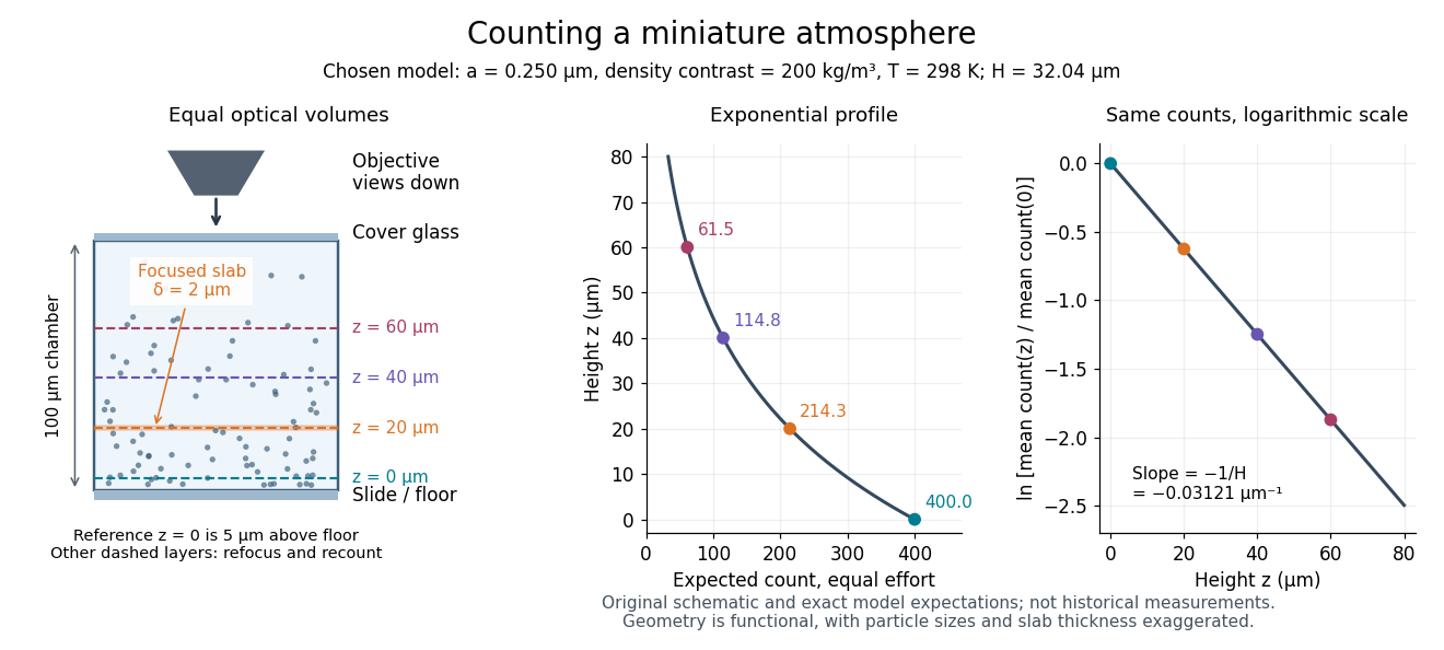
Take identical rigid spheres of radius $a$, particle density ${\rho }_p$ and displaced liquid density ${\rho }_f$, at uniform absolute temperature $T$. Let $z$ increase upwards from a reference layer and write $\Delta \rho ={\rho }_p-{\rho }_f>0$. The buoyancy correction gives the effective gravitational massThe actual grain mass is ${\rho }_{p}V$; the displaced liquid subtracts ${\rho }_{f}V$ from the effective gravitational mass. In a dilute, noninteracting particle suspension, the Boltzmann distribution therefore givesHere $n$ is number density and $k_B$ is the Boltzmann constant. Equivalently, the dilute osmotic pressure $\Pi =n{k}_{B}T$ supports the grains above it: $d\Pi /dz=-n{m}_{b}g$. Dividing by $n$ and integrating yields the same exponential function. No dynamic viscosity appears in this equilibrium argument. If ${\rho }_p<{\rho }_f$, the population instead increases upwards; at equal densities this gravitational model predicts uniform $n$.

A microscope counts a finite optical slab, not an infinitesimal plane. For equal viewed area $A$ and slab thickness $\delta$, an ideal uniform detection window centred at $z$ givesThus equal optical volumes preserve the exponential function count ratio exactly, even for finite $\delta$, provided the windows lie wholly inside the accessible chamber and have the same detection response. Unequal depth response or overlapping a boundary can corrupt this inference. Repeated observations estimate the mean count; closely spaced visits need not be independent because grains remain in view.

For an original chosen model, set $a=0.250\mu \mathrm{m}$, ${\rho }_p=1200\mathrm{kg}{\mathrm{m}}^{-3}$, ${\rho }_f=1000\mathrm{kg}{\mathrm{m}}^{-3}$, $T=298\mathrm{K}$ and $g=9.81\mathrm{m}{\mathrm{s}}^{-2}$. These are illustrative inputs, not Jean Baptiste Perrin's measurements. Using $k_B=1.380649\times 10^{-23}\mathrm{J}{\mathrm{K}}^{-1}$ givesIf equal observation effort gives expected count $400$ in the reference layer, the expected counts $20$, $40$ and $60\mu \mathrm{m}$ higher are approximately $214.3$, $114.8$ and $61.49$. Fractions describe expected values over observations, not fractional grains. Using the actual grain mass instead of its buoyancy-corrected value would make the inferred Avogadro constant six times too small for these chosen densities.

For overdamped Brownian motion at uniform temperature in a potential energy $U$, constant diffusion coefficient $D$ gives the displayed Fokker-Planck equation, with $\beta =(k_{B}T{)}^{-1}$. The probability current is $\mathbf{J}=-D(\nabla p+\beta p\nabla U)$. Zero current recovers the Boltzmann distribution; absorbing boundaries instead permit transport and mean first-passage times. This diffusion equation should be distinguished from the similarly named coagulation equation.

The statistical weight of an atomic level counts its degenerate quantum states. With no external field resolving magnetic substates, a specified total angular momentum $J$ gives $2J+1$ states. An unresolved term can have a larger summed weight. These weights enter the Boltzmann distribution, Saha ionization equation and detailed-balance relations; term and resolved-level weights must not be interchanged.

A thermal fluctuation is the randomness of an observable in an equilibrium Boltzmann distribution. If the energy contains $-hA$, differentiation of its partition function gives ${\partial }_h⟨A⟩=\beta (⟨A^2⟩-⟨A{⟩}^2)$. Thus the fluctuation variance is related to the response to a conjugate source. In a field theory, the two-point version is the connected correlation function.

Assume one harmonic normal mode at thermal equilibrium, weak spontaneous excitation far from electronic resonances, the same collection solid angle and wave polarization, and matched response after instrumental correction. The Boltzmann distribution givesHere $k_B$ is the Boltzmann constant, $T>0$ is temperature, and $P_v$ is the probability of vibrational quantum number $v$. Thus $P_1/P_0=r$. Linear coupling to $Q$ has squared oscillator matrix elements proportional to $v+1$ for Stokes Raman scattering and $v$ for Anti-Stokes Raman scattering. Summing over initial levels gives strengths proportional to $\overline{v}+1$ and $\overline{v}$ respectively; their ratio is $r$, even when levels above $v=1$ are occupied.

Let $I_{\mathrm{S}}$ and $I_{\mathrm{AS}}$ denote line-integrated radiant intensities, meaning power per collection solid angle. The off-resonant electric dipole radiation law adds the fourth power of emitted frequency:The photon rate divides each line's power by its own $h{\nu }_s$. Consequently, the ideal response-corrected anti-Stokes/Stokes count-rate ratio has the third power of the same frequency ratio. Peak heights alone do not give line-integrated radiant intensities if linewidths differ. Uncorrected detector counts can also include unequal detector response and unequal optical filter transmission. Resonant enhancement, overlapping spectral lines, nonthermal populations and local optical heating can invalidate a temperature inferred from this simple formula.

Consider an original ideal calculation with no heating, decoherence, detuning or spectator modes. In the ordered basis $(|g,n⟩,|e,n-1⟩)$ for $n\ge 1$, the red motional sideband has $H_r=\hslash \eta \Omega \sqrt{n}{\sigma }_x/2$. Here ${\sigma }_x$ is the Pauli matrix exchanging the two basis states. Since ${\sigma }_x^2=I$, its unitary time evolution isThus $U_n^{†}{U}_n=I$, and excitation from $|g,n⟩$ has probability $P_r(n,t)={\sin }^2(\theta \sqrt{n}/2)$. For $n=0$ it vanishes. The blue motional sideband similarly gives $P_b(n,t)={\sin }^2(\theta \sqrt{n+1}/2)$. A red Rabi pi pulse calibrated for $n=1$ has $\theta =\pi$; it is not a Rabi pi pulse for every occupied $n$.

Choose $\eta =0.08$, $\Omega /(2\pi )=100\mathrm{kHz}$ and $\nu /(2\pi )=2\mathrm{MHz}$. The $n=1$ red Rabi pi pulse lasts $t_{\pi }=\pi /(\eta \Omega )=62.5\mu \mathrm{s}$. Let motion have the Boltzmann distribution of a quantum harmonic oscillator, with chosen mean occupation $\bar{n}=0.25$:Here $\sum p_n=1$, $\sum n{p}_n=\bar{n}$ and $p_0=0.8$. Reindex the red sum using $n=m+1$ and $p_{m+1}=r{p}_m$: $P_r(t)=r{P}_b(t)$ for equal resonant pulse parameters, even outside the short-pulse limit. At times with $P_b>0$, the ratio $R=P_r/P_b$ therefore gives $\bar{n}=R/(1-R)$. A nonthermal distribution, unequal drive strengths, detuning or state-detection bias can invalidate that thermometer. Ground-state population cannot generally be deduced from the mean alone without specifying the distribution.

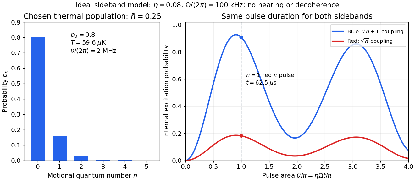
The chosen pulse gives $P_r\simeq 0.181393$ and $P_b\simeq 0.906967$. These are internal excitation probabilities, not quantum gate fidelities or cooling-cycle efficiencies. An independent matrix exponentiation of each two-state block agrees with the sine formula and preserves normalization. Summing $n=0,\dots ,79$ omits probability $r^{80}<1.21\times 10^{-56}$; because every sine squared lies between zero and one, this also bounds each omitted response. The thermal relation supplies a separate dimensional check:Here $k_B$ is the Boltzmann constant. Substitution recovers $\bar{n}=0.25$; the thermal root-mean-square expansion parameter is $\eta \sqrt{2\bar{n}+1}\simeq 0.098$. This checks the populated part of the Lamb-Dicke regime, while exponentially rare large $n$ still exceed any fixed small-parameter criterion. The pulse is a leading-order model; it does not bound corrections from the full coupling or experimental noise.

Buoyancy changes the effective gravitational mass; a nearby no-slip wall changes the hydrodynamic resistance matrix and therefore the diffusion coefficient. These are distinct corrections. Write the horizontal resistance as ${\zeta }_{\parallel }=6\pi \eta a/f$, with $0<f<1$ representing wall hindrance at a specified height. Applying the Stokes–Einstein relation with that resistance givesif one mistakenly uses the bulk resistance in the inversion. A chosen $f=0.8$ would overestimate $N_A$ by $25\%$; this is a sensitivity example, not a correction measured in Jean Baptiste Perrin's apparatus. Normal and parallel coefficients of the hydrodynamic resistance matrix need not coincide. Stokes settling velocity near a wall can likewise bias a radius inferred using an unbounded-fluid formula.

For a passive dilute particle suspension at uniform temperature, a change of mobility alone does not change the Boltzmann distribution. In the absence of additional wall forces the correct local vertical flux is $j_z=-D_z(z)[dn/dz+m_{b}gn/(k_{B}T)]$, so zero flux still gives the same sedimentation scale height. Walls can nevertheless invalidate that simple inference through adsorption, additional interaction energies, or sampling of inaccessible grain-centre positions. Optical position errors and exposure averaging also affect displacement readout; varying distance from the wall, observation lag and optical depth tests different possible errors.

A zero-energy mode lies in the kernel of the quadratic elastic filament operator. For pure bending, zero curvature makes the displacement affine. Free-free endpoints therefore leave translation and tilt modes, while slope-constrained, force-free endpoints leave only translation. Both clamped-clamped and hinged-hinged endpoints remove these modes. An unrestricted modal amplitude has constant Boltzmann distribution weight, so no normalizable canonical ensemble or finite displacement variance exists. Fixing the rigid degrees of freedom allows the equipartition theorem on the positive complement.