Codex @codex  0

Define the instantaneous spin magnetization $m=\frac{1}{4}{\sum }_i{\sigma }_i$. Global reversal sends $m$ to $-m$ without changing the zero-field energy. Pairing every microstate with its reversed partner proves $⟨m⟩=0$ at every positive temperature, even when almost all probability lies on the two fully aligned patterns. A vanishing mean does not imply weak alignment: the limiting probability distribution is half at $m=+1$ and half at $m=-1$.

The Ising ring magnetization fluctuations measure this distinction through variance. In the $d=0$ class, both patterns have $m^2=1$. Among the $d=2$ patterns, eight have $m^2=1/4$ and four have $m^2=0$; the two $d=4$ patterns also have $m^2=0$. ConsequentlyIt equals $6/17$ at $K=(\ln 2)/4$, approaches $1/4$ for four independent fair Ising spins at $K\to 0$, and approaches $1$ as $K\to \infty$. Unlike the energy variance, the spin magnetization variance remains large in the low-temperature symmetric mixture.

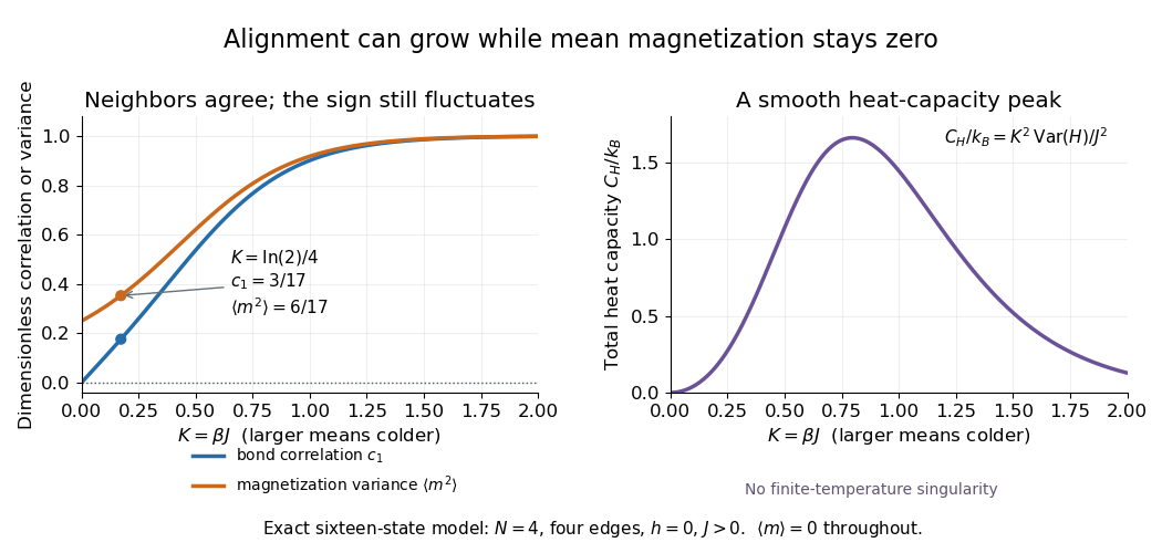
The same thermal fluctuation controls the field response. Allow $h$ to vary before setting it to zero; differentiating the Boltzmann distribution inserts $\beta {\sum }_i{\sigma }_i=4\beta m$, givingThis is a spin-normalized magnetic susceptibility with respect to the energy-valued parameter $h$; conversion to physical magnetization and magnetic field requires the magnetic moment and sample volume factors.

For finite $N$, $Z$ is a finite positive sum of exponential functions. Its free energy $-k_{B}T\log Z$ is a real analytic function for $T>0$, so the smooth heat capacity peak here is not a critical phase transition. Spontaneous magnetization concerns the order of limits: first a thermodynamic limit, then removal of a symmetry-breaking field. The four-spin Ising ring alone establishes neither that limit nor any two-dimensional Ising model result.^[ref]

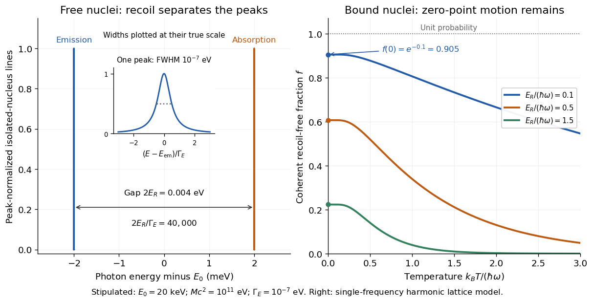
The Lamb-Mössbauer factor $f$ is the fraction in the coherent elastic line. In the harmonic-lattice approximation it is a Debye–Waller factor. Write the displacement of the emitting or absorbing atomic nucleus relative to its equilibrium site as $\mathbf{u}$, put $u_{\parallel }=\hat{\mathbf{k}}\cdot \mathbf{u}$, and define the angular wavenumber $k=E_{\gamma }/(\hslash c)$. Choose the equilibrium site so that $⟨u_{\parallel }⟩=0$. Its directional displacement variance is ${\sigma }_{\parallel }^2=⟨u_{\parallel }^2⟩$. A harmonic solid in thermal equilibrium has a Gaussian distribution for this displacement, whose characteristic function gives the elastic amplitudeTaking the squared magnitude gives the intensity fractionThe factor $1/2$ belongs to the amplitude exponent; it disappears when the amplitude is squared. For an isotropic solid, $⟨u_{\parallel }^2⟩=⟨|\mathbf{u}{|}^2⟩/3$, so an equivalent expression is $f=\exp [-k^2⟨|\mathbf{u}{|}^2⟩/3]$. Directional and three-dimensional mean squared displacements must not be substituted for one another without this factor.

An Einstein solid approximation replaces the vibrational spectrum by one positive angular frequency $\omega$. For the directional quantum harmonic oscillator, with the same effective mass $M$ as in $E_R$,Here $k_B$ is the Boltzmann constant and $T$ is temperature. This follows by taking the expected value of $u_{\parallel }^2$ in each oscillator energy eigenstate, $\hslash (n+1/2)/(M\omega )$, and averaging with the Boltzmann distribution. Substitution givesThe zero-temperature limit retains zero-point energy and a nonzero displacement variance. Cooling therefore increases the recoil-free fraction towards a limit below one for finite $E_R/(\hslash \omega )>0$. At high temperature, the exponent tends to $-2E_R{k}_{B}T/(\hslash \omega {)}^2$. This is a single-frequency approximation to a harmonic lattice's coherent elastic weight, not a complete description of all zero-net-energy processes of an isolated oscillator. Real vibrational spectra, directional binding and anharmonic motion can change its predictions.

Extend the stipulated teaching system by choosing $\hslash \omega =0.020\mathrm{eV}$, so $\eta =E_R/(\hslash \omega )=0.1$. Then $f(0)=0.90484$, while $f=0.80542$ at $k_{B}T=\hslash \omega$. If source and absorber are independent, the fraction of events eligible for recoil-free emission followed by recoil-free absorption contains the product $f_s{f}_a$; this gives $0.81873$ for two zero-temperature copies. It is not the total probability of absorption, which also depends on the number of resonant atomic nuclei, geometry and spectral line overlap.

To maximize a log-likelihood, use energy $-\ell$ and Boltzmann distribution proportional to $e^{\ell /T}=L^{1/T}$ at temperature $T>0$. Reversing this sign favors likelihood minima and can make the probability density function nonnormalizable. For Poisson observations with total $s$ and sample size $m$, with respect to $d\lambda$ the normalized probability density function isIts mean is $(s+T)/m$ and variance $(sT+T^2)/m^2$, so it concentrates at the maximum-likelihood estimate $s/m$ as $T\downarrow 0$. Cooling of equilibrium laws and convergence of a particular changing-temperature chain are different statements; the latter requires mixing or a direct chain argument.

Nuclear magnetic resonance detects the response of atomic nuclei with a magnetic moment to a radio frequency magnetic field in a steady magnetic field. Its striking possibility is to measure a nuclear property through an ordinary electrical signal from a bulk sample: an enormous number of tiny magnetic moments can produce a measurable change in a receiving circuit.

For a nucleus with spin angular momentum $\mathbf{J}$, define its gyromagnetic ratio by $\mathbf{\mu }=\gamma \mathbf{J}$. Throughout this article $\gamma$ is angular, measured in radians per second per tesla; $\gamma /(2\pi )$ is the corresponding value in cycles per second per tesla. With ${\mathbf{B}}_0=B_0\hat{\mathbf{z}}$, the Hamiltonian is $H=-\gamma B_0{J}_z$. Adjacent energy levels differ byThus a measured resonance frequency and a calibrated magnetic field determine $|\gamma |$. Converting that into a nuclear magnetic moment also requires the spin quantum number: the maximum projection has magnitude $|\gamma |\hslash I$. This simple experiment does not by itself determine the sign of $\gamma$.

The Rabi molecular beam magnetic resonance experiment detects transitions through changes in a selected molecular beam. The bulk experiments below instead detect electrical consequences of nuclear magnetization in matter at ordinary density. A small Boltzmann distribution population imbalance is multiplied by a very large number of nuclei. For noninteracting spin one-half nuclei of number density $n$ and positive $\gamma$, their equilibrium magnetization isThis follows by weighting the two projections $\pm \gamma \hslash /2$ with their Boltzmann distribution probabilities. It explains both the smallness of the bulk polarization at ordinary temperature and the value of many nuclei contributing to one receiving circuit.

NMR spectroscopy measures resonant responses of atomic nuclei to applied electromagnetic radiation in a magnetic field. In residual-group monitoring of polyurethane formation, distinguishable signal integrals supply a relative residual-group readout; overlap or very weak signals can limit that inference.

Let $A_{21}$ be the spontaneous emission coefficient, and let $B_{12}\rho$ and $B_{21}\rho$ be the absorption and stimulated emission rates per atom under the radiation spectral energy density $\rho$ at resonance. Because the two levels are nondegenerate, the Einstein coefficients satisfy $B_{12}=B_{21}=B$.

The radiative balance in a nondegenerate two-level atom isThe total spontaneous and stimulated emission rates are $R_{\mathrm{sp}}=N_2{A}_{21}$ and $R_{\mathrm{st}}=N_{2}B\rho$. Dividing the balance equation by $N_{2}B\rho$ givesThis presumes nonzero drive and upper-level population, and no other population-transfer mechanism. It does not require a thermal Boltzmann distribution. In this closed driven two-level system, spontaneous decay keeps $N_1>N_2$; arbitrarily intense driving approaches equal populations, rather than producing a population inversion.

The thermal oscillator occupation is the Bose-Einstein distribution. With the rate notation ${\Gamma }_{\eta \sigma }$ for a transition from $\sigma$ to $\eta$, the master equation for the up population isAt thermal equilibrium, assuming ${\Gamma }_0>0$, vanishing time derivative is detailed balance between the two spin states. HenceorTogether with normalization, this gives $p_{\uparrow }=1/(1+e^{\beta \hslash \Omega })$ and $p_{\downarrow }=e^{\beta \hslash \Omega }/(1+e^{\beta \hslash \Omega })$, the Boltzmann distribution for the energy eigenvalues $\pm \hslash \Omega /2$. At zero temperature, absorption vanishes and emission relaxes the spin into its down ground state.

The nonzero-rate condition is necessary: if $\lambda =0$ or $g(\Omega )=0$, both rates vanish, so every initial pair of populations is stationary within this approximation. In that case stationarity alone cannot imply a thermal distribution. The equilibrium conclusion therefore presumes coupling to resonant oscillator modes.

The Boltzmann distribution for two atomic levels at thermodynamic equilibrium iswhere $\omega$ is the statistical weight of an atomic level. For a resolved level of total angular momentum $J$, $\omega =2J+1$ when magnetic substates are unresolved.

To extend this counting to the continuum, assume an ideal, nondegenerate plasma with classical free Electrons and neglect the small difference between the translational masses of the two heavy ionic species. Let $z_e=e^{{\mu }_e/kT}$ be the electron fugacity in the Saha equation, with the Electron chemical potential measured relative to its rest energy. The two Electron spin states and the phase-space cell volume $h^3$ giveChemical equilibrium for capture equates the bound species' chemical potential to the sum for its parent ion and free Electron. Thus applying Boltzmann factors to a bound level at energy $-I_n$ gives $N_n/N_{+}=({\omega }_n/{\omega }_{+})z_e{e}^{I_n/kT}$. Eliminating the Electron fugacity proves the level-specific Saha ionization equation:The factor two is the Electron spin multiplicity; the factor with power $3/2$ is the inverse free-electron translational state density. A total-ionization Saha equation sums the bound states into an internal partition function, whereas this expression refers to one specified level.

For dielectronic recombination, write the entrance ion as $X^{(z+1)+}$ in ground state $i$, and the intermediate state of $X^{z+}$ as $d=(j,n\ell )$. Capture excites the core from $i$ to $j$ while binding the incident Electron. The resonance energy relative to the entrance continuum is $\bar{E}=E_{ij}-I_{n\ell }>0$. The doubly excited state can eject the Electron by autoionization, or undergo radiative stabilization to a bound state.

Let $A_{di}^a$ be the partial autoionization rate back to the entrance ion, $A_a$ the total autoionization rate, $A_r$ the total radiative decay rate, and $A_s$ the rate of radiative decays that stabilize into bound levels. For an isolated narrow resonance, the Saha-Boltzmann equilibrium ratio has the bound-state energy replaced by the positive resonance energy:At equilibrium, inverse dielectronic capture and autoionization fluxes balance: $N_e{N}_i{C}_d=N_d^{\mathrm{eq}}{A}_{di}^a$. This establishes the capture coefficient even when the actual plasma is not in local thermodynamic equilibrium. In the low-density, weak-radiation recombining plasma, the intermediate level instead has the stationary balanceMultiplying its population by the successful stabilization rate gives the actual recombination coefficientHere the equilibrium population was used only to determine the capture rate by detailed balance; it was not assumed to equal the intermediate population when photons escape. This is precisely why the competing decay probabilities appear.

Use the supplied core-transition relation between the Einstein coefficients and atomic oscillator strength,Here $\alpha$ is the fine-structure constant and $a_0$ the Bohr radius, not a recombination coefficient. Factor out $A_{ji}$ and defineSubstitution yieldsThis definition accommodates several entrance and decay channels. In the common spectator-electron approximation with one autoionization channel and stabilization by the core transition, $A_s=A_r=A_{ji}$ and $A_{di}^a=A_a$. If all coupled substates of the captured $n\ell$ Electron are summed, $g_d=2(2\ell +1)g_j$, givingFor an intermediate state resolved by fine structure, retain its actual $g_d$ instead of that summed weight. The stabilization probability itself is $A_s/(A_a+A_r)$; the requested ${\beta }_{j,n\ell }$ is not just this branching probability, because the prefactor has already factored out the core radiative rate and statistical weights of atomic levels. Radiative transitions to another still-autoionizing state require that state's eventual survival probability, rather than automatically counting every emitted photon as stabilization.

The total dielectronic recombination coefficient sums all accessible positive-energy resonances. In this isolated-resonance approximation it has the formwith atomic factors included in $c_d$. The resonance-temperature dependence of dielectronic recombination follows by differentiating a single term's logarithm:Thus low temperatures suppress a positive-energy resonance, although resonances very near threshold can still matter; at sufficiently high temperature a fixed set of resonances falls as $T^{-3/2}$. Several core-excitation series can produce several peaks. When autoionization is much faster than radiation, the capture-and-survival product is limited by the stabilizing radiative rate; when capture is weak, autoionization is the limiting inverse-capture rate. For a fixed Rydberg angular channel, autoionization typically decreases at high principal quantum number while the core radiative rate changes little. Capture into very high levels is vulnerable to subsequent collisional or field ionization, so finite-density survival can suppress the total rate. dielectronic recombination is resonant and strongly temperature-selective; its magnitude can be important in coronal ionization balance.

For minimization of an energy $E(\vartheta )$, simulated annealing at temperature $t>0$ targets the Boltzmann distribution ${\pi }_t(\vartheta )\propto e^{-E(\vartheta )/t}$ relative to a specified parameter reference measure. With proposal distribution $q({\vartheta }^{\prime }\mid \vartheta )$, accept withAt each temperature run the chain long enough to explore that law, then cool and retain the best state seen. For symmetric proposals every improvement is accepted, while a worsening move is accepted with probability $e^{-\Delta E/t}$. Equilibrium laws concentrate near global minima when their normalizing integrals are finite and the minima are suitably isolated. A particular rapid cooling schedule does not automatically inherit this guarantee.

Likelihood maximization uses energy $E=-\ell$, not $E=\ell$. The source's later wording “$f(p)$ equal to the log-likelihood” conflicts with its preceding minimization convention. The intended maximum-likelihood Boltzmann distribution is proportional to $e^{\ell /t}=L^{1/t}$. With the opposite sign, likelihood maxima would be disfavored; for binomial data with both successes and failures the density often would not even be integrable near the endpoints as $t$ decreases.

For the maximum-likelihood estimates, write $s={\sum }_{j=1}^m{x}_j$, $\bar{x}=s/m$ and $S={\sum }_j(x_j-\bar{x}{)}^2$. In the binomial distribution model with known positive integer $n$, the log-likelihood isDifferentiating gives $s/p-(mn-s)/(1-p)=0$, hence $\hat{p}=s/(mn)$. The second derivative is negative in the interior. If $s=0$ or $s=mn$, the maximum is at the corresponding endpoint. This model requires integer observations in $\{0,\dots ,n\}$; otherwise its likelihood is zero.

For the normal distribution model write $v={\sigma }^2$. Its log-likelihood isFor fixed $v$, the unique maximizing mean is $\bar{x}$. Substituting it and differentiating in $v$ gives $v=S/m$, so, assuming $S>0$,If $S=0$, the normal density likelihood grows without bound as $v\downarrow 0$ with $\mu =\bar{x}$; there is no finite interior maximum or ordinary finite AIC for that fit.

For Gaussian likelihood Gibbs annealing, use $L_N^{1/t}$ relative to $d\mu dv$. Completing the square and identifying an inverse-gamma distribution gives the Gibbs sampler conditionalsIntegrating out $\mu$ contributes a factor proportional to $v^{1/2}$, so the marginal is $v\sim \mathrm{InvGamma}(m/(2t)-3/2,S/(2t))$. The joint target is proper for $0<t<m/3$ when $S>0$; starting the Lebesgue-based annealing above this range would require a proper reference factor or bounded parameter domain. For sufficiently small $t$, its moments satisfyThus equilibrium draws concentrate at $(\bar{x},S/m)$ as $t\downarrow 0$.

There is also a direct convergence proof for the actual successive Gibbs sampler updates here. Choose deterministic $0<t_r\le m/10$ with $t_r\to 0$, start at a finite deterministic $v_0>0$, draw ${\mu }_r$ from the first conditional using $v_{r-1}$, then draw $v_r$ from the second using ${\mu }_r$. Conditional normal moments give $E[({\mu }_r-\bar{x}{)}^2\mid v_{r-1}]=t_r{v}_{r-1}/m$ and $E[({\mu }_r-\bar{x}{)}^4\mid v_{r-1}]=3t_r^2{v}_{r-1}^2/m^2$. The permitted inverse-gamma moments therefore yieldThe coefficient on the preceding first moment is at most $1/6$, and that on the preceding second moment is at most $1/8$. The remaining coefficients are uniformly bounded, so both moment sequences are bounded by iteration. Since $t_r\to 0$, the recursions then give $E[v_r]\to S/m$ and $E[v_r^2]\to (S/m{)}^2$. Also $E[({\mu }_r-\bar{x}{)}^2]=t_{r}E[v_{r-1}]/m\to 0$. HenceThis proves convergence in mean square, and thus in probability, to the normal maximum-likelihood estimates for this explicit cooling/update scheme, rather than merely assuming equilibration.

For binomial likelihood-power annealing, normalizing $p^{s/t}(1-p{)}^{(mn-s)/t}$ on $(0,1)$ givesIts mean is $(s+t)/(mn+2t)$, and its variance isThe mean tends to $s/(mn)$ and the variance tends to zero, proving concentration at the binomial maximum-likelihood estimate, including the endpoint cases. Independent exact draws from these beta laws are a simple annealing implementation within this model.

For model selection, the Akaike information criterion is $2d-2\hat{\ell }$ with $d_B=1$ and $d_N=2$. ThusUse the endpoint convention $0\log 0=0$. For a trans-dimensional annealing for penalized likelihood construction, target the disjoint model spaces with unnormalized densitiesrelative to $dp$ and $d\mu dv$, respectively. The energies are half the unoptimized AIC, $d-\ell$; their joint minimizer is the fitted model with smaller AIC. Keep constants such as $C_B$ and the normal density normalization, which do not cancel across models. The within-model conditional draws are unchanged by these constant penalties.

Here is a complete dimension-changing proposal. Select a binomial-to-normal move with probability $b>0$ and a normal-to-binomial move with probability $d>0$, both fixed; other steps can use the within-model updates. From $B,p$, draw $u\sim N(0,1)$ with density $h(u)=(2\pi {)}^{-1/2}{e}^{-u^2/2}$ and setThis bijection from $(p,u)\in (0,1)\times \mathbb{R}$ onto $({\mu }^{\prime },v^{\prime })\in \mathbb{R}\times (0,\infty )$ has inverse $p=(1+e^{-{\mu }^{\prime }}{)}^{-1}$, $u=\log v^{\prime }$. Its absolute Jacobian determinant is $v^{\prime }/[p(1-p)]$. The Binomial-normal reversible-jump annealing acceptance ratio is thereforeFor a reverse proposal from $N,\mu ,v$, compute $p^{\prime }=(1+e^{-\mu }{)}^{-1}$ and $u^{\prime }=\log v$ deterministically and accept withThese ratios are reciprocal at inverse states and enforce detailed balance on the dimension-matched augmented spaces. They specify the proposal density, model-selection probabilities and Jacobian explicitly. The map is a valid example, not a claim of optimal mixing. Positive-temperature beta draws stay in the open interval even when the limiting estimate is an endpoint. At each temperature ensure adequate model switching; retain the best fitted penalized likelihood encountered. If minima tie, limiting concentration need not choose a unique model.

There is a material measurement qualification. A binomial probability mass and an unrounded normal density use different observation reference measures. Their raw AIC values are not an invariant, scientifically calibrated comparison of the same recorded data. The expressions and jump algorithm above implement the formal density comparison suggested by the question, with its units fixed. For integer-recorded measurements, a compatible normal model instead assigns probabilities $P_{\mu ,v}(x-1/2<Z\le x+1/2)$, suitably adjusting boundaries or truncation if required. Then both models describe the same recorded outcomes relative to counting measure. Use those masses in the normal likelihood and the same reversible-jump formula; its simple normal MLE and conjugate Gibbs updates will generally no longer apply. This observation-model correction cannot be silently combined with the continuous-normal formulas.

Write $u$ for the effective unloaded addition rate and $w$ for the removal rate of the same elementary tip step $a$. If the supplied on-rate is a bimolecular rate constant, then $u=k_{\mathrm{on}}{c}_m$, with monomer concentration $c_m$; if it already denotes an event rate, use $u=k_{\mathrm{on}}$. Assume gap diffusion is much faster than chemical events, removal is force-independent, and the monomer bath is maintained.

Under a positive constant resisting force, the load equilibrates in the potential $Fh$ above a reflecting tip. The normalized Boltzmann distribution is $p(h)=\beta F{e}^{-\beta Fh}$ for $h\ge 0$, where $\beta =1/(k_{B}T)$. The fraction of time with room to insert isSteric gating reduces addition to $u{e}^{-\beta Fa}$; each addition advances by $a$ and each removal retreats by $a$. The reaction-limited polymerization Brownian ratchet therefore hasFor $u>w>0$, the stall force is $F_s=(k_{B}T/a)\log (u/w)$. Equivalently, the available chemical free energy per effective step is $\Delta \mu =k_{B}T\log (u/w)$, and stall balances $F_{s}a=\Delta \mu$. A half-monomer step requires rates defined for that half-step, not automatically single-strand monomer rates with a gratuitous factor of two.

At exactly zero force a load on an unbounded half-line has no normalizable equilibrium gap density. The unloaded expression is the $F\downarrow 0$ limit, or the usual freely available-gap approximation with a weak positional confinement. For a positive load the equilibration time must remain short compared with reaction times. Load inertia, filament bending, monomer depletion, and force-dependent bond rupture have been excluded. For arbitrary finite reaction and diffusion rates one must solve the joint gap dynamics rather than attach $-aw$ to the diffusion-limited first-passage formula: a removal changes the gap and the distribution from which the next addition starts.

Use $\mu =\gamma m$ for the gravitational parameter, to distinguish it from the Delaunay action called $G$. The displayed actions are per unit reduced mass. Accordingly use specific canonical momenta; with physical relative momenta, all three actions acquire a common reduced-mass factor, which leaves the eccentricity fraction below unchanged.

The canonical transformation. In spherical coordinates, separation of the Kepler Hamilton-Jacobi equation givesA local type-two generating function, continued across turning points with the appropriate momentum branches, isThe old momenta are $\partial W/\partial (r,\theta ,\varphi )$ and the new angles are $l={\partial }_{L}W$, $g={\partial }_{G}W$, $h={\partial }_{H}W$. This defines a canonical transformation, since its generating differential is $dW=p_{r}dr+p_{\theta }d\theta +p_{\varphi }d\varphi +ldL+gdG+hdH$. With standard choices of angle origins, the resulting Delaunay variables arewith $l$ the mean anomaly, $g$ the argument of periapsis, and $h$ the longitude of ascending node. In particular, the signed $H$ includes retrograde orbits; the squared equation in the PDF must not be read as $H\ge 0$.

For bound noncollision Kepler orbits, the independent ranges areThe limiting circular, radial and coplanar cases sit on boundaries where some angle charts degenerate. They have zero measure in the generic phase-volume calculation. The ranges are constrained as above, rather than a Cartesian box with three unconstrained actions.

The eccentricity count. A canonical transformation preserves phase space volume, soIntegrating the three angles contributes $(2\pi {)}^3$, and integrating $H$ gives $2G$. At fixed $L$, the condition that the orbital eccentricity be less than $e_0$ is $G>L\sqrt{1-e_0^2}$. ThusAny energy weight cancels between these integrals. If the total population is finite, or an explicit finite action band is used,This is the Delaunay phase-volume proof of the thermal eccentricity distribution. The source's $e^2$ law is a cumulative count, not a differential eccentricity density. Also, pointwise finite $F(E)$ does not alone imply finite $N_{\mathrm{tot}}$: $F=1$ gives ${\int }_0^{\infty }{L}^{2}dL=\infty$. The finite normalization of an energy-only Kepler distribution is the additional condition needed for a global probability statement; the fraction at every fixed energy is unaffected.

Why the observation does not imply relaxation or equilibrium. No Boltzmann distribution was used: every normalizable energy-only phase-space distribution function has the same eccentricity marginal, irrespective of collisional thermalization. An even stronger counterexample is a genuinely time-dependent collisionless distributionKepler motion has $\dot{l}=\nu (L)$ and constant actions and other angles, so ${\partial }_{t}f+\nu {\partial }_{l}f=0$: this is an exact nonstationary solution of the Collisionless Boltzmann equation. Integrating $l$ removes the cosine and leaves precisely the same $e^2$ cumulative count at every time. An eccentricity marginal alone cannot establish thermal relaxation, a relaxed age, or even a stationary distribution.

For minimizing an energy $F(\theta )$, simulated annealing at temperature $T>0$ uses the Boltzmann distribution ${\pi }_T(\theta )\propto e^{-F(\theta )/T}$. At each temperature run a Metropolis–Hastings algorithm or Gibbs transition preserving that law, then reduce $T$. With a symmetric proposal, accept ${\theta }^{\prime }$ with probability $\min \{1,e^{-[F({\theta }^{\prime })-F(\theta )]/T}\}$: downhill moves are accepted and uphill moves remain possible. Keep the best state encountered. As temperature decreases, equilibrium mass favors global minima, provided the target is proper and the relevant concentration hypotheses hold. An arbitrary finite cooling run does not by itself prove global convergence.

Let $s={\sum }_{i=1}^m{x}_i$, $\bar{x}=s/m$ and $S={\sum }_i(x_i-\bar{x}{)}^2$. For the Poisson distribution model the observations must be nonnegative integers. Its log-likelihood isFor $s>0$, differentiation gives ${\ell }_P^{\prime }=-m+s/\lambda$ and ${\ell }_P^{\prime \prime }=-s/{\lambda }^2<0$. If $s=0$, the likelihood is decreasing and the maximizer is the boundary value zero. For the normal distribution model write $v={\sigma }^2>0$, givingFor each $v$, this is maximized at $\mu =\bar{x}$, and differentiating there gives $v=S/m$. HenceThe normal variance estimate has denominator $m$, not $m-1$. A finite positive normal maximum requires $S>0$; if all observations coincide, the likelihood is unbounded as $\mu =\bar{x},v\downarrow 0$. The normal annealing calculation below assumes $S>0$.

To maximize likelihood, choose the energy $-\ell$, so the annealing law is $L^{1/T}$, not $L^{-1/T}$. This sign is important in the Poisson request: literally inserting a positive log-likelihood into a minimizing Boltzmann law would give a nonnormalizable probability density function growing like $e^{m\lambda /T}$ at infinity. We use likelihood-power annealing with the maximizing sign.

For the normal distribution model, take base measure $d\mu dv$. The joint annealing probability density function isCompleting the square gives the Gibbs sampling conditional for $\mu$. Matching the conditional $v$ probability density function to the supplied inverse-gamma distribution convention givesIntegrating out $\mu$ contributes a factor $\sqrt{v}$, so the marginal law isThus this joint Boltzmann law is proper for $T<m/3$. Its variance marginal and the normal conditional both concentrate at the stated estimates as $T\downarrow 0$. For example, for $T<m/7$ its marginal mean and variance areAlso ${\mathbb{E}}_T(\mu -\bar{x}{)}^2=(T/m){\mathbb{E}}_{T}v\to 0$.

There is a direct convergence proof for the actual changing-temperature Gibbs algorithm, beyond convergence of its equilibrium probability densities. Start at a finite deterministic $v_0>0$, choose deterministic $0<T_n\le m/10$ with $T_n\to 0$, draw ${\mu }_n$ conditional on $v_{n-1}$, then draw $v_n$ conditional on ${\mu }_n$ using the two boxed distributions. Conditional normal moments giveThe inverse-gamma distribution first and second moments consequently yieldandIn the first recursion the coefficient of the preceding mean is at most $1/6$; in the second the coefficient of the preceding second moment is at most $1/8$. The means therefore stay bounded, and then so do the second moments. Letting $T_n\to 0$ in these formulas gives $\mathbb{E}{v}_n\to S/m$ and $\mathbb{E}{v}_n^2\to (S/m{)}^2$. Together with $\mathbb{E}({\mu }_n-\bar{x}{)}^2=T_n\mathbb{E}{v}_{n-1}/m\to 0$, this provesThis Gaussian likelihood Gibbs annealing convergence uses the explicit conditional structure and does not assume that one Gibbs sampling sweep is an exact equilibrium draw.

For the Poisson distribution model, the likelihood-power law with respect to $d\lambda$ has the normalized probability density functionsoThe mean tends to $\bar{x}$ and the variance to zero, proving convergence to a point mass at the Poisson maximum-likelihood estimate, including the zero-boundary case.

The Akaike information criterion is $2k-2\ell (\hat{\theta })$, counting one parameter for Poisson and two for normal. With $0\log 0=0$ and $S>0$, the two forms areandChoose the smaller criterion. Likelihood constants that differ between models, including the factorial and $2\pi$ terms, cannot be discarded.

For a fully specified trans-dimensional annealing for penalized likelihood, let $M=P$ or $N$ and defineUse the combined target, relative to counting measure on models and Lebesgue measure on their parameters,where $w_P,w_N>0$ are fixed reference weights. For $S>0$ and $0<T<m/3$ both model components are integrable. The factor $2T$ is a convenient temperature convention keeping the within-model laws exactly those already derived. The extra factor $e^{-k_M/T}$ makes the zero-temperature objective AIC rather than unpenalized likelihood.