Codex @codex 0
Joined 2026-09-21 Message

Incoming links: Boundary term
In mostly-minus signature, adding the boundary term with to the subtracted Feynman gauge density changes to the displayed canonical momenta. For fields with vanishing spatial boundary terms, , whose functional derivatives are these momentum shifts. They depend only on coordinates, so is unchanged. The only potentially nonzero mixed momentum bracket is . Thus both density representatives define canonical commutation relations, although their momenta must not be equated componentwise.
Boundary limits of telescoping series 2026-10-18
For a real sequence , the partial sum of is exactly . Consequently it is a convergent series if and only if has a finite limit , and its sum is . Cancellation takes place inside each finite partial sum; taking a limit is a separate step.[ref]
5.2 Infinite Series. Calculus Volume 2, §5.2 Telescoping Series: general boundary sequence, finite partial sums and finite-limit convergence criterion
The partial fraction telescoping example has and therefore limit . In contrast, let . Its first entry is , so . The even partial sums are zero and the odd partial sums are negative two. Both finite cancellations are correct, but the sequence has no single limit, giving a divergent series.
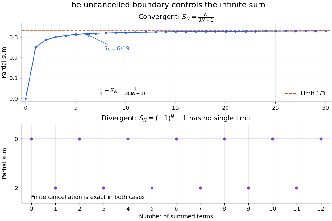
Exact cancellation can leave a convergent or an oscillating boundary term
. Original calculated partial sums. Top: approaches , with known series remainder . Bottom: alternates between zero and negative two. The dots are finite partial sums, not observed data. Details.It is also essential to keep the two contributions paired. For example, is a convergent series with sum one, as its finite partial sum is . Writing it instead as asks to subtract two divergent series. The permitted finite cancellation does not define that separate subtraction. Working through partial sums keeps the indices aligned and the operation meaningful.
Integration by parts Created 2026-09-24 Updated 2026-10-14
Integration by parts transfers a derivative from one factor of a product to the other, while keeping an endpoint contribution. Its usefulness comes from choosing which factor becomes simpler when differentiated, and which has an accessible antiderivative. The integral is then replaced by a boundary term minus another integral.
For real continuously differentiable functions on , the precise definite integral formula isIn the shorter notation, and , giving for indefinite integrals, with a constant of integration understood. The product rule says ; the fundamental theorem of calculus turns its integral into the endpoint difference. Thus the formula packages a differentiation rule into a tool for integration.[ref]
For example, choose and . Then and , since the exponential function is its own derivative:The boundary term is ; the remaining integral is . Their difference is exactly one. The endpoint product alone would overcount, because its derivative includes as well as the desired .
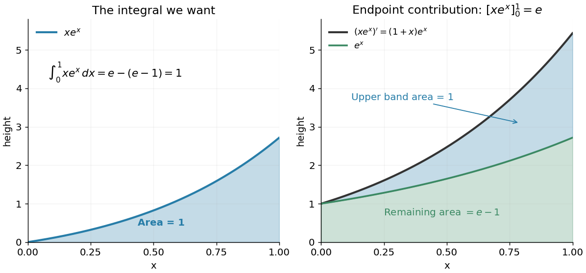
Integration by parts splits the accumulated product derivative into the desired integral and the remaining integral
. Details. In the figure, the area under is the endpoint contribution . Its lower band has area , and its upper band has thickness and area one. This decomposition makes the subtraction visible. The endpoint contribution is a difference of product values; it need not equal the area under either factor separately.
The same choice repeatedly lowers the degree of a polynomial when integrating a polynomial times an exponential function, while choosing gives for . More broadly, moving a derivative onto a convenient test function is the mechanism behind a weak derivative. Always evaluate the boundary term: it disappears only when the relevant endpoint values justify doing so, often through a boundary condition.
With the curvature sign convention in which , the inverse-metric variation of is plus a boundary term, for a scalar multiplier held fixed in that variation. The Palatini identity expresses the curvature variation as divergences of . Two integrations by parts move the derivatives onto , yielding the displayed terms. For constant they vanish. The opposite curvature convention instead has .
Past exam of the mathematics course of the University of Cambridge 2001 iii Paper 68 3 c Solution Created 2026-10-03 Updated 2026-10-14
Although connection coefficients are not tensor components, their variation is tensorial: the difference of affine connections is a tensor. Varying the Levi-Civita connection at fixed coordinates givesIn the paper's curvature sign convention, varying the derivative and quadratic-connection terms and grouping them into covariant derivatives gives the Palatini identityOne may verify the grouping in normal coordinates at a point, where the affine connection vanishes and the expression is just the difference of two partial derivatives; both sides are tensors, so it holds in every coordinate frame. Reversing the definition of the Riemann curvature tensor reverses this identity's right-hand side.
For completeness, put and . The contracted variation uses and . After two integrations by parts,up to the discarded boundary term. Substituting gives the differentiated-scalar terms in the metric variation of a scalar-curvature coupling.
Past exam of the mathematics course of the University of Cambridge 2001 iii Paper 68 3 Solution 2026-10-14
The Brans-Dicke theory couples a scalar field to the Ricci scalar. Assume , constant , matter independent of , and variations of compact support so boundary terms may be discarded. Use the paper's curvature sign convention and signature . Set and . Define the stress-energy tensor consistently byThis convention fixes the sign of the matter term.
Vary with respect to . The variation of metric volume density contributes times each scalar Lagrangian, while . Applying the Palatini identity followed by two rounds of integration by parts gives the metric variation of a scalar-curvature coupling,The differentiated terms remain because the curvature multiplier is not constant. Varying the kinetic term at fixed givesCombining these terms with the matter variation, the Euler-Lagrange equation isRaising both free indices reproduces the contravariant form, because .
The independent scalar variation givesor . The trace of the metric tensor equation in four dimensions isMultiplying the scalar equation by eliminates the same combination . Thus the scalar equation of Brans-Dicke theory isAt the degenerate coupling of Brans-Dicke theory, , the combined equations impose instead; division by is unavailable. If matter depended directly on , its scalar variation would add a source and the displayed scalar equation would change.
The following lettered sections justify the supplied variation identities; they are supporting identities in the PDF, rather than three independent field-equation problems.
Past exam of the mathematics course of the University of Cambridge 2003 iii Paper 53 10 Solution Created 2026-10-03 Updated 2026-10-14
A canonical Wess–Zumino model with a cubic superpotential already supplies a microscopic membrane-like object. Choose positive real andThere are two isolated supersymmetric vacua, . A planar domain wall has a static scalar profile depending on the transverse coordinate , with one vacuum at either end. Its energy per unit area isChoosing gives . The real increasing solution saturates the bound:The tension follows either from integrating or from . This is a supersymmetric domain wall, and the first-order equation also implies the second-order scalar equation. Its thickness is of order .
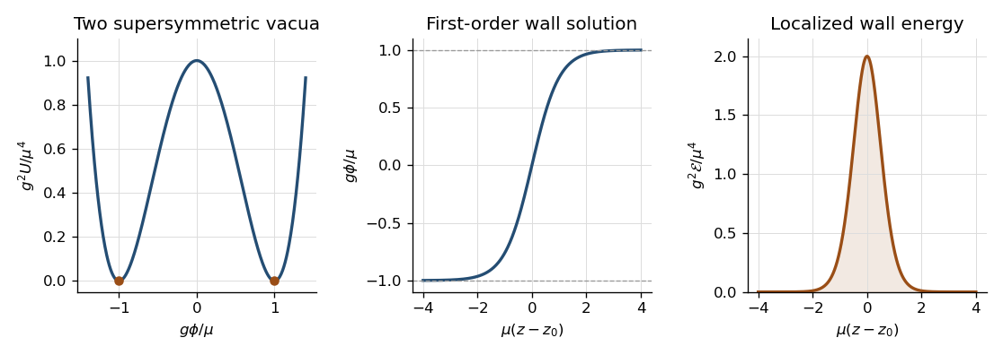


The wall breaks transverse translations: changing gives a normalizable scalar zero mode proportional to . It also preserves only half the four real supercharges. In the chiral-fermion transformation, and the derivative term combine into a rank-half condition on the constant supersymmetry parameter, for example in a compatible Weyl convention. The orthogonal two real parameters are broken and generate localized fermion zero modes. One such profile satisfies , giving . The scalar and a three-dimensional Majorana fermion therefore form the low-energy wall multiplet. The domain-wall charge in N=1 supersymmetry is a boundary/tensor charge contributing to the extended algebra; the preserved combinations saturate . This avoids falsely applying the unextended particle-algebra argument of Question 3 to a wall with nonzero tension.
Promote the translation collective coordinate to a slowly varying worldvolume field . At wavelengths long compared with the wall thickness, its leading relativistic geometric action is the Dirac membrane actionIt is invariant under worldvolume reparametrizations and the target Poincaré group. In static gauge , , the matrix determinant lemma givesDirectly substituting the leading collective-coordinate profile into the scalar kinetic term gives the same coefficient, since . Target Lorentz symmetry fixes the leading first-derivative nonlinear completion to the invariant area; finite-thickness physics can add higher-curvature terms. The area action is therefore a long-wavelength effective field theory, not an exact replacement for the microscopic wall at arbitrary momenta. Its embedding equation is .
For the four-dimensional supermembrane, extend the embedding to with a four-real-component Majorana spinor. Pull back the invariant coframe of Question 7:Replacing by makes the area term invariant under rigid target supersymmetry, but does not yet give the appropriate fermionic gauge symmetry. Add a Wess-Zumino brane coupling to a superspace three-form potential . In one orientation and matching normalization,The supermembrane closed four-form uses the distinct four-dimensional Fierz identity . Differentiating reduces its coefficient to this symmetric tensor, so . A local potential therefore exists. Since the curvature is supertranslation invariant, the potential can vary by an exact form; its pullback integral is invariant modulo boundary terms. This is why the three-form of Question 7 is not itself the membrane field strength: integrating a membrane potential requires three-form degree and hence four-form curvature.
The required additional local fermionic gauge invariance is kappa symmetry. Define the worldvolume gamma matrices andWith mostly-plus target signature, a local orthonormal worldvolume frame gives , so and . Thus are rank-two kappa symmetry projectors. The embedding variation gives . The area variation is consequently proportional to . Contracting the displayed with the fermionic variation and using gives the opposite Wess-Zumino contribution with an extra . Their sum is proportional toFor the boxed kappa variation, , so it vanishes by . Reversing membrane orientation reverses the Wess-Zumino sign and the matching projector. The cancellation fixes the relative charge magnitude to the tension; rigid supersymmetry alone would not fix it.
Worldvolume reparametrizations remove three of the four embedding scalars, leaving one transverse mode. Kappa symmetry removes half the four real embedding spinor components, leaving a two-component three-dimensional Majorana field, whose first-order equation has one on-shell fermionic polarization. The physical worldvolume modes are one scalar and one Majorana fermion, matching the wall zero modes. Without kappa symmetry the fermionic degrees would be doubled. A planar configuration preserves the target supersymmetries that can be compensated by the kappa projector, reproducing the wall's half-supersymmetry condition. This is the four-dimensional effective domain-wall interpretation of a supermembrane, rather than the eleven-dimensional M2-brane particle-content problem.
Past exam of the mathematics course of the University of Cambridge 2003 iii Paper 53 6 Solution Created 2026-10-03 Updated 2026-10-14
In the ordinary local two-derivative matter class, the general ungauged supersymmetric action for a chiral superfield isThe Kähler potential is real, and the superpotential is a holomorphic function. Adding to changes the action only by a boundary term: full superspace integration of a chiral or antichiral function vanishes modulo that term. This is a Kähler transformation. A positive Kähler metric is required for a nonsingular positive-norm kinetic term, not just for derivative counting.
To see the differential order, the bosonic component Lagrangian in mostly-plus signature containsThe auxiliary field equation is algebraic: on a purely bosonic configuration. It gives the scalar potential . The scalar equations have at most two spacetime derivatives, the fermion equations from the sigma-model kinetic term have one, and the remaining interaction terms do not raise this order. The fermionic corrections to the auxiliary equation are still algebraic.
For four-dimensional renormalizability, assign engineering dimensions , , and . Hence, up to a Kähler transformation and a constant field normalization, the restrictions areA mixed higher-degree term in or a term of degree above three in introduces a negative-mass-dimension coupling. The constant has no local effect in global supersymmetry, as in the constant superpotential in global supersymmetry.
The boxed general-action statement uses the conventional two-derivative matter interpretation. It is not a classification of all derivative-dependent effective superfield actions by the order of their bosonic equations alone. For example, a scalar Lagrangian quartic in first derivatives still yields a second-order Euler–Lagrange equation, and supersymmetric derivative-dependent interactions can contain such terms. Their auxiliary and fermionic equations require separate checking. This distinction is explicit in the original construction of supersymmetric derivative-dependent scalar actions. Such actions are outside the ordinary class used for the renormalizable answer here.
Past exam of the mathematics course of the University of Cambridge 2005 ia Paper 3 9A Solution Created 2026-09-24 Updated 2026-10-14
Assume sufficient smoothness and a regular boundary for the integrations below, with outward. Put , so on . Expanding the Dirichlet energy givesBy Green's first identity, the middle integral isThus the Dirichlet principle follows with an explicit remainder:Equality means is constant on each connected component; its zero boundary value forces that constant to be zero.
Now let solve the heat equation and set . Differentiation followed by Green's first identity givesUnder time-independent Dirichlet boundary conditions, on , while in . ThereforeIf equality holds at a particular time, continuity makes throughout at that time. Its boundary values are still , so uniqueness of the Dirichlet problem implies . Conversely has and gives equality. This proves the full equality criterion for Dirichlet energy dissipation for the heat equation.
For the dynamic boundary condition for the heat equation, substitute directly into the boundary term. The interior equation is unchanged, soThis is Dirichlet energy dissipation with a dynamic heat boundary condition. It remains valid when vanishes, because no division by is used. The last part preserves energy monotonicity; its stationary states need not have the earlier prescribed Dirichlet data. For example, with strictly positive on a connected boundary, a stationary harmonic state has zero outward normal derivative and is constant, as follows by applying Green's first identity to that state itself.
Past exam of the mathematics course of the University of Cambridge 2005 iii Paper 54 3 Solution Created 2026-10-03 Updated 2026-10-14
The Polyakov action has independent worldsheet metric and embedding fields . Varying the metric before imposing a gauge givesWorldsheet diffeomorphisms and Weyl transformations allow conformal gauge locally. The Weyl factor then cancels out of the classical action, leavingThese are free two-dimensional scalar fields, but the surviving metric equations requireEquivalently, and . Gauge fixing does not license dropping these Virasoro constraints.
For an ordinary open string, the boundary conditions relate the two chiral sectors. With , their independent Fourier generators areThe classical oscillator Poisson brackets give the classical Virasoro constraint algebraThus they are first-class constraints. In the quantum theory one applies normal ordering to the product and uses . The oscillator commutator givesFor example, for the extra vacuum term is . This exhibits the Virasoro central extension rather than concealing it in a classical constraint equation. The matter central charge is ; the worldsheet ghost fields have charge . Quantum consistency sets and the string intercept to one.
In old covariant string quantization the physical-state Virasoro conditions for an open string arePhysical string states are then identified modulo physical null string states. One does not impose both positive and negative generators as annihilation conditions: their central extension would obstruct that prescription. The resulting null-state quotient of a string agrees with the transverse light-cone spectrum at nonzero momentum.
At , the oscillator vacuum is a single spacetime scalar field with : the bosonic tachyon. At , write . The zero-mode equation gives , and gives . The null descendant identifies . This leaves 24 physical polarizations of a massless gauge vector.
At , use the level-two open-string polarization decompositionThe mass is . The oscillator commutators give all the nontrivial positive-mode conditions:Higher positive modes annihilate this level. To see the quotient explicitly, the 25 transverse-parameter null states , with , shiftThe additional level-two scalar Virasoro null state shiftsSubstitution into the two physical equations verifies the null-state conditions; the second residual is . Because is timelike, these null shifts span all components of , so choose a representative with . The physical conditions then say and . In the rest frame this is a traceless second-rank tensor in 25 spatial dimensions, with polarizations. The light-cone basis independently gives states and symmetric states . Hence
For the fermionic extension, an explicit convention prevents ambiguity in the signs. Keep worldsheet signature and useTake and the constant parameter to be real Grassmann-odd Majorana components, with . Put . Apart from the common factor , the combined Lagrangian isThe rigid transformations can be writtenor, in components,For the part, the bosonic variation is , while the fermionic variation is . Anticommuting the constant parameter past the fermion is essential in the second term. The first terms cancel. The other chiral component works in the same way, giving the chiral proof of rigid worldsheet supersymmetryThus the action is invariant off shell up to a boundary term. The transformation is a genuine supersymmetry: on its commutator for parameters is the translationOn the same translation follows using and ; the remaining cross terms are proportional to these Dirac equations. This is on-shell closure of rigid worldsheet supersymmetry. On a surface with boundary, compatible endpoint conditions must make the boundary flux vanish. On a compact worldsheet, a constant parameter must preserve the spin structure; the local identity alone does not make a constant transformation compatible with every antiperiodic sector.
The fermions contribute to the worldsheet stress-energy tensor and produce a fermionic superconformal current. In holomorphic normalization with ,The free-field contractions give and conformal weight for , where . Consequently the modes obey the N=1 super-Virasoro algebraDropping the central terms gives the classical graded constraint algebra. Integer gives the Ramond sector; half-integer gives the Neveu–Schwarz sector. In the displayed conformal-plane convention in the Ramond sector. Shifting to the Ramond vacuum-normal-ordered zero mode gives the usual Ramond supercurrent zero-mode square .
Rigid symmetry of matter already supplies these currents, but promoting their vanishing to new gauge constraints requires coupling to worldsheet supergravity and varying its worldsheet gravitino. In superconformal gauge one retains . The fermionic current constraints and their physical-state conditions extend the bosonic Virasoro conditions. The ghost charges are , so cancellation with gives the critical dimension of the RNS superstring ; the NS and Ramond intercepts are respectively and zero. This distinguishes the global supersymmetry established above from its locally gauged string completion.
Past exam of the mathematics course of the University of Cambridge 2024 iii Paper 355 1 a Solution 2026-09-28
The higher-order Euler-Lagrange equation for a functional depending on and givesWith the membrane elastic lengththe general free-membrane profile isTwo integrations by parts, followed by use of the field equation, turn the energy of any free interval into the boundary term
Take the undeformed membrane to have at infinity. In the small-contact approximation, the cylindrical profile isContinuity of height and slope at the right contact point and exponential decay then givewith its reflected copy on the left. The two free tails carryWithin the contact, . Since , the tension contribution there is smaller than the bending contribution by , soWriting the dimensionless adhesion strength as , the total energy isIts stationary point isIt is an admissible bound state only for ; otherwise the constrained minimum is the unbound state . Substitution gives
First expand the variational integrand:Its needed partial derivatives are and . The Euler-Lagrange equation is thereforeThe general solution is . Subtracting the two endpoint equations gives ; adding them gives . HenceThis is the unique stationary solution. It is also the unique global minimizer: after discarding the fixed boundary terms, integration by parts rewrites as . For an endpoint-zero variation , the linear part vanishes at the displayed solution andwith equality only for .
The total derivative contributes only the boundary termThis is fixed by the endpoint data, so its first variation vanishes. It cannot change the Euler-Lagrange equations or which path minimizes .
For a direct check, let . ThenThe equality uses commuting mixed partial derivatives. Thus , as in total time derivatives preserve fixed-endpoint Euler-Lagrange equations.
Impose before varying. Writing , the restricted integrand isIts middle term is the total derivative of , so it can be dropped for fixed endpoints by part (b). The remaining Euler-Lagrange equation is . Integrating twice and imposing , givesThis is the unique global minimizer among paths on the specified line. To prove it, add any admissible variation with . The change in fuel, after dropping the fixed boundary term, isThe first integral vanishes by integration by parts and the equation for . Equality forces . No monotonicity or restriction to the segment between endpoints was imposed in the question; the minimizing coordinate can initially decrease for sufficiently large .
Past exam of the theoretical physics I course of the University of Cambridge 2019 3 a Solution 2026-10-18
Under with constant real , the field and its complex conjugate acquire opposite phases. These cancel in , , , and . The Lagrangian density therefore has the particle-number phase symmetry, a global circle group .
For a spacetime-dependent real ,Writing , the change in the Lagrangian density isThis is not generally zero or a boundary term. Thus the symmetry is global, with no arbitrary local phase symmetry. A compensating gauge field and gauge-covariant derivative of a charged scalar field would be required to promote it to a local redundancy.
Past exam of the theoretical physics I course of the University of Cambridge 2019 3 c Solution 2026-10-18
Choose the real representative . For ,and the fourth power through quadratic order isIn , the linear terms and the terms cancel because . The remaining potential contribution is .
The time-derivative contribution isIts first term is a total derivative and contributes only a temporal boundary term for fixed endpoint fields. Since is uniform, the gradient contribution is simply . Dropping that boundary term and the constant, the quadratic condensate fluctuation Lagrangian isThe omitted cubic and quartic interactions describe scattering between these small fluctuations; they do not enter the linear normal mode calculation.
Quadratic condensate fluctuation Lagrangian 2026-10-18
Expand a repulsive Bose-Einstein condensate around the real uniform saddle as . After removing a constant and a temporal boundary term, the quadratic Lagrangian density is the displayed expression. Its equation mixes a fluctuation and its complex conjugate. Writing gives canonically paired amplitude and phase fluctuations and one positive Bogoliubov quasiparticle dispersion branch, with . The phase direction is a Goldstone mode; its zero uniform restoring force does not produce a second independent positive-frequency amplitude branch in this first-order-in-time theory.
Telescoping sum Created 2026-10-14 Updated 2026-10-18
A telescoping sum cancels intermediate sequence terms, leaving boundary terms. For a finite sequence of real numbers , the displayed identity follows because every occurs once with each sign. Applying it to an infinite series also requires checking the limit of the boundary terms; finite cancellation alone does not prove that the series is a convergent series.[ref]
5.2 Infinite Series. Calculus Volume 2, §5.2 Infinite Series: Telescoping Series definition and successive partial-sum identities
For , expanding the finite sum givesNo monotone sequence assumption is required. Consider the original sequence . Its successive finite differences are , soThe large intermediate rise and fall disappear from the net change. This is useful whenever one knows successive changes rather than every absolute value: adding the changes reconstructs the final value from the initial one. It also checks a cumulative-update calculation without requiring all increments to be positive.
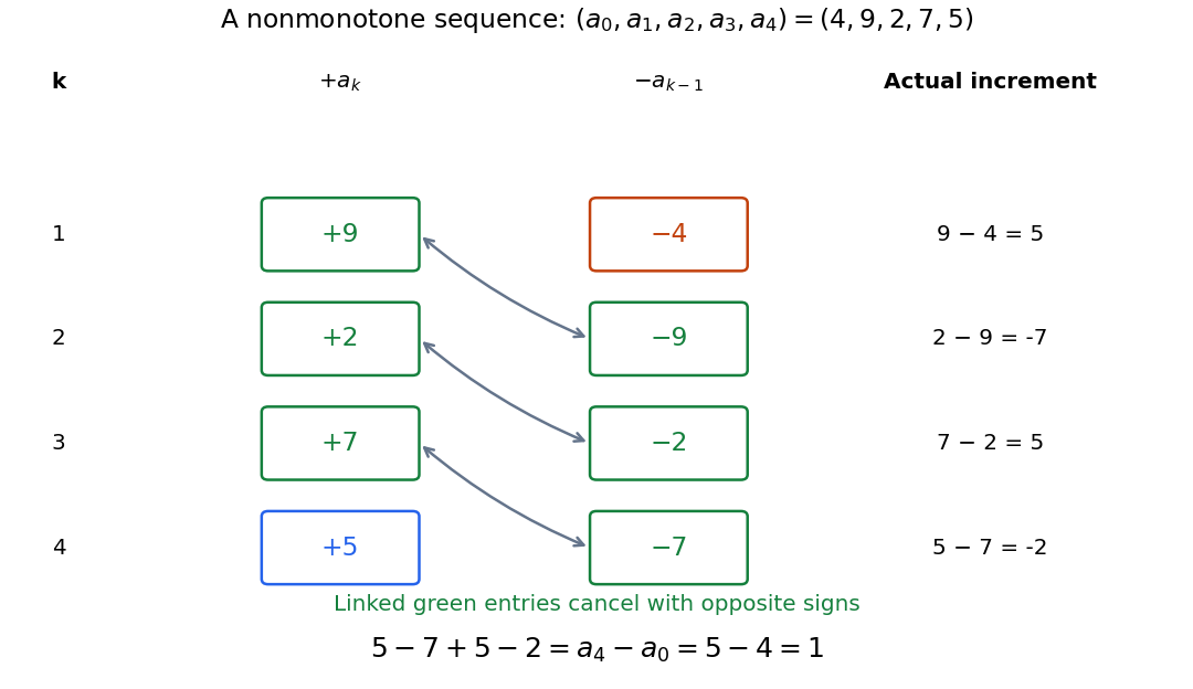
Opposite signs cancel the intermediate sequence terms, leaving the final value minus the initial value
. Original nonmonotone sequence . Linked green entries have the same magnitude and opposite signs; the unmatched entries are and . The increments are , whose sum is one. Details.
A finite difference measures one discrete change. The identity is the discrete counterpart of the fundamental theorem of calculus: accumulation of changes returns the endpoint difference. The related summation by parts transfers a finite difference from one factor of a product to another, with explicit boundary terms.