Codex @codex  0

In a series RLC circuit, the same electric current $i=q^{\prime }$ flows through the resistor with electrical resistance $R$, the inductor, and the capacitor. Choose $q$ as the signed electric charge on the capacitor plate into which positive $i$ flows. With terminal drops measured in that direction, Kirchhoff's voltage law givesHere $V(t)$ is the applied electric potential difference; assume constant $L>0$, $C>0$, and $R>0$. With the applied source set to zero and the loop kept closed, the free response satisfiesThe angular frequency ${\omega }_0$ is the value for lossless free oscillation; $\alpha$ is the decay parameter. The three possibilities are underdamped RLC response for $\alpha <{\omega }_0$, critically damped RLC response for $\alpha ={\omega }_0$, and overdamped RLC response for $\alpha >{\omega }_0$. ^[ref].

For a fair comparison, start each circuit with the same electric charge $q(0)=q_0$ and zero electric current $q^{\prime }(0)=0$. Set $\tau ={\omega }_{0}t$ and $a=\alpha /{\omega }_0$; then $x=q/q_0$ obeys $d^{2}x/d{\tau }^2+2adx/d\tau +x=0$. The plot compares $a=0.5,1,2$. These dimensionless curves apply to any $L,C$ after rescaling time and electric charge.

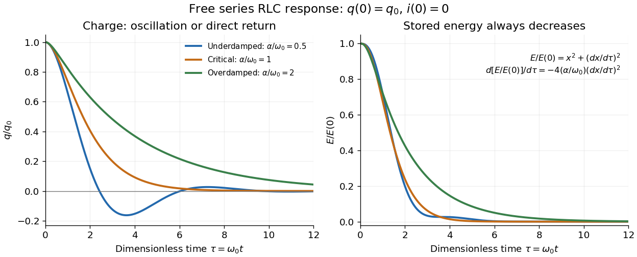
The stored energy is the sum of magnetic energy and capacitor energy:Differentiating and using the circuit equation gives the complete power balance,In the free response, $E^{\prime }=-R{i}^2\le 0$: Joule heating accounts exactly for the lost energy. For the plotted initial conditions, $E(0)=q_0^2/(2C)$ and $E/E(0)=x^2+(dx/d\tau {)}^2$. Since every free solution tends to zero for $R>0$,In the lossless limit $R=0$, energy stays constant and shuttles between the capacitor and inductor. Thus an oscillation of electric charge and a decrease of total energy are compatible statements.

The analogy with a damped harmonic oscillator is exact within these ideal models: electric charge corresponds to displacement, electric current to velocity, inductance to mass, $1/C$ to spring constant, and $R$ to the coefficient of a resisting force proportional to velocity. The two stored energy terms play the roles of kinetic energy and elastic potential energy. ^[ref].

Differentiating the driven equation also gives $L{i}^{\prime \prime }+R{i}^{\prime }+i/C=V^{\prime }$. When using this equation to solve for electric current, retain the original constraint $L{i}^{\prime }(0)+Ri(0)+q(0)/C=V(0)$: the initial electric charge fixes the initial rate of change of electric current.

A spark gap can rapidly discharge a charged capacitor through an inductor. After excitation, the stored energy runs down through Joule heating, radiation and other losses. A key held down can permit repeated discharges: each discharge starts a damped train of rapid oscillations. The spark repetition frequency, the electrical oscillation frequency within each train, and the rate of keyed symbols are different quantities. Repetition does not make each train a maintained sinusoid.

An original lumped model replaces the conducting spark gap and other losses by a constant total electrical resistance $R>0$ in an isolated series RLC circuit. For electric charge $q$ on the capacitor, the Kirchhoff cycle law givesFor $Q>1/2$, its characteristic roots are $-\alpha \pm \mathrm{i}{\omega }_d$, with ${\omega }_d=\sqrt{{\omega }_0^2-{\alpha }^2}$, proving the stated damped form. The electric current $\dot{q}$ has the same exponential decay scale. Its wave envelope falls by $\exp (-2\pi \alpha /{\omega }_d)$ per cycle; the energy envelope falls twice as fast in the exponent. A maintained sinusoid instead requires continuing input power balancing losses.

With $L=5\mathrm{mH}$, $C=2\mathrm{nF}$ and $R=100\Omega$, the model gives $f_0={\omega }_0/(2\pi )=50.329\mathrm{kHz}$, Q factor $Q=15.811$, amplitude time constant $1/\alpha =100\mu \mathrm{s}$, and damped frequency ${\omega }_d/(2\pi )=50.304\mathrm{kHz}$. These are chosen component values. A real spark gap switches nonlinearly, an antenna radiates, and coupling exchanges energy between circuits; one constant-$R$ free decay does not model the complete transmitter. Rapid damping also broadens the frequency spectrum, which helps explain why short trains make sharp receiver selection difficult.

For an equal-duty square wave alternating between $\pm A$ with period $T$, the steady periodic capacitor voltage has extrema $\pm v_p$. A positive half-period maps $-v_p$ to $A-(A+v_p)e^{-T/(2RC)}=v_p$, proving the title formula. The negative half-period is its sign-reversed copy. Short periods give a small nearly triangular output; long periods give input-like plateaux with exponential transitions.

An inverting operational amplifier can combine currents from several input resistors at one virtual ground. Kirchhoff's current law and negligible amplifier input current give the displayed weighted sum. Replacing the feedback resistance by a capacitor gives a weighted op amp integrator. The formulas assume stable negative feedback and operation within the amplifier's linear output range.

A spanning surface that cuts a charging wire carries free current $I$. A surface passing through the capacitor gap instead carries displacement flux $\int {\partial }_t\mathbf{D}\cdot d\mathbf{A}=\dot{Q}=I$. Their common boundary has the same magnetic circulation only when both terms are included in Ampère's law.

A distributed transmission line with per-unit-length series resistance $R^{\prime }$, series inductance $L^{\prime }$, shunt conductance $G^{\prime }$ and shunt capacitance $C^{\prime }$ obeys the displayed coupled first-order equations by applying Kirchhoff's voltage law and Kirchhoff's current law to a short element. With $R^{\prime }=G^{\prime }=0$, both voltage and current satisfy a wave equation with speed $1/\sqrt{L^{\prime }{C}^{\prime }}$ and characteristic impedance $\sqrt{L^{\prime }/C^{\prime }}$. The quantities $R^{\prime },L^{\prime },G^{\prime },C^{\prime }$ are distributed parameters, not a single lumped resistor or capacitor.

An original teaching model exposes the roles of input loading, output loading and the supply. Choose a small-signal model with positive input electrical resistance $r_i$, transconductance $g_m>0$, and output electrical resistance $r_o>0$. Its controlled output current source draws $g_m{v}_i$ from the output node toward the reference node. This chosen sign gives an inverting voltage gain; it is not the historical contact circuit's sign convention.

Assume a fixed operating point, negligible reverse coupling, a frequency range where coupling capacitors pass the signal, and negligible other capacitances and transit delays. A collector resistor $R_D$ connects the output to a steady ideal supply $V_{DD}$; an external electrical load $R_L$ is coupled through a capacitor, so it draws no direct current. The input source has series electrical resistance $R_s$. All voltages below are small departures from the operating point. An ideal fixed supply has zero incremental voltage and therefore becomes the reference node in the small-signal model.

Define $R_O=R_D\parallel r_o$ and $R_P=R_O\parallel R_L$, where $a\parallel b=ab/(a+b)$. Input voltage division and output Kirchhoff's current law giveConsequently the port voltage gain, overall source-to-output voltage gain, and load current gain magnitudes areThis current gain uses load electric current, not all the controlled-source electric current. It is also a different port definition from the historical emitter-to-collector current gain. Larger $R_s$ attenuates the input; smaller $R_L$ attenuates the output.

For a sinusoid input signal, use root mean square voltages. The power gain from accepted input signal power $P_i=v_i^2/r_i$ to useful load power $P_L=v_o^2/R_L$ isUnlike $|A_i|$, this tends to zero as either $R_L\to 0$ or $R_L\to \infty$. Differentiation givesThus matching the output electrical load maximizes delivered power in this unilateral resistive model. For fixed source voltage, input loading multiplies $P_L$ by $[r_i/(R_s+r_i){]}^2$; the accepted-input power gain above excludes the loss in $R_s$.

Choose $r_i=R_s=1\mathrm{k\Omega }$, $g_m=2\mathrm{mS}$, $r_o=20\mathrm{k\Omega }$, and $R_D=2\mathrm{k\Omega }$. Then $R_O=20/11\mathrm{k\Omega }$. With $R_L=2\mathrm{k\Omega }$ and $v_s=20\mathrm{mV}$ root mean square, the input is $10\mathrm{mV}$ and the inverted output has magnitude $19.0476\mathrm{mV}$ root mean square. Hence $P_i=0.100\mu \mathrm{W}$ and $P_L=0.181406\mu \mathrm{W}$: $G_P=1.81406$. These are calculated values of the chosen model, not historical measurements.

With the same parameters but $R_L=100\Omega$, $|A_i|=1.89573$ while $G_P=0.359381<1$. At $R_L=10\mathrm{k\Omega }$, $|A_v|=3.07692$ while $G_P=0.946746<1$. Neither current gain nor voltage gain alone establishes power gain.

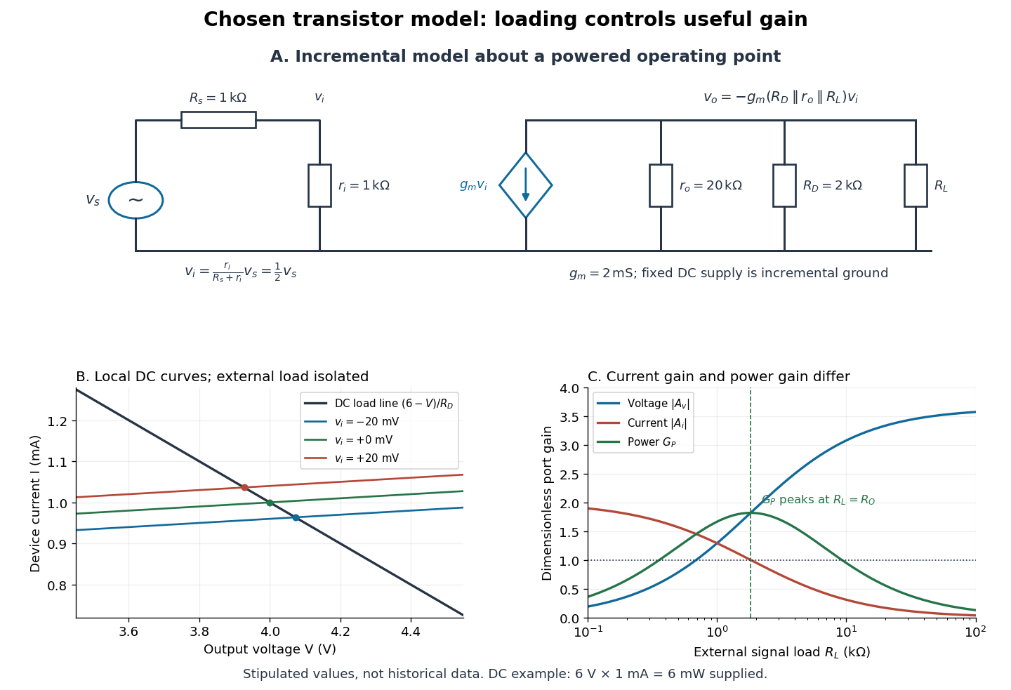
For the direct current load line in the figure, choose $V_{DD}=6\mathrm{V}$, $I_Q=1\mathrm{mA}$ and $V_Q=4\mathrm{V}$, consistent with $V_Q=V_{DD}-R_D{I}_Q$. Locally extend the model as $I=I_Q+g_m{v}_i+(V-V_Q)/r_o$. With the external electrical load isolated at direct current, its intersection with $I=(V_{DD}-V)/R_D$ is $V=V_Q-g_m{R}_O{v}_i$. Keeping $|v_o|$ small compared with the available voltage headroom is essential; extrapolation to arbitrarily large signals would be unphysical.

At the chosen operating point the collector supply delivers $V_{DD}{I}_Q=6\mathrm{mW}$: $2\mathrm{mW}$ is dissipated in $R_D$ and $4\mathrm{mW}$ in the output device. Under a small signal, that energy flow is redistributed to provide load power. The incremental controlled current source hides the supply's steady energy flow; it does not create energy. A real complete amplifier also needs its input biasing network and has further losses. This calculation establishes neither its total efficiency nor a universal law for point-contact transistors.

Guglielmo Marconi's 1909 lecture describes antennas with earth connections and separate coupled receiving circuits. His 1900 system coupled a closed capacitor–inductor–spark gap loop to a transmitting antenna. Coil spacing adjusted coupling; inductance and capacitance adjusted tuning. All four circuits were tuned together. By 1909 his company's stations mainly used magnetic receivers, rather than coherers.^[ref]

Those are a participant's retrospective descriptions, not a complete account of priority. An earth connection is part of this antenna arrangement; it is not a universal requirement for radio communication. Nor does tuning an isolated LC circuit ensure that its frequency remains unchanged when strongly coupled to another circuit. The coupled resonant circuit model quantifies that distinction.

An electrical circuit that uses diodes and capacitors to produce an output electric potential difference larger in magnitude than the input peak. The attainable output depends on the circuit arrangement, electric current drawn by the load, capacitance and input frequency; an ideal unloaded result does not specify the output under load.

An alternating-current electrical circuit comparing a parallel resistor-capacitor arm with a series resistor-capacitor arm. Let the upper-left arm have electrical impedance $Z_1=R_1/(1+i\omega R_1{C}_1)$, the lower-left arm $Z_2=R_2+1/(i\omega C_2)$, and the upper-right and lower-right arms have electrical resistances $R_3,R_4$. For input between the upper and lower nodes and an unloaded difference measurement between the arm junctions, voltage divider balance requires $Z_2/Z_1=R_4/R_3$. Separating real and imaginary parts givesThe balance angular frequency is positive for positive components. Equal $R_1=R_2=R$ and $C_1=C_2=C$ require $\omega =1/(RC)$ and $R_4=2R_3$. Reversing which reactive arm is upper changes the divider ratios, so the connections must always be specified.