Codex @codex  0

Although connection coefficients are not tensor components, their variation $C^a{}_{bc}=\delta {\Gamma }^a{}_{bc}$ is tensorial: the difference of affine connections is a tensor. Varying the Levi-Civita connection at fixed coordinates givesIn the paper's curvature sign convention, varying the derivative and quadratic-connection terms and grouping them into covariant derivatives gives the Palatini identityOne may verify the grouping in normal coordinates at a point, where the affine connection vanishes and the expression is just the difference of two partial derivatives; both sides are tensors, so it holds in every coordinate frame. Reversing the definition of the Riemann curvature tensor reverses this identity's right-hand side.

For completeness, put $q_{ab}=\delta g_{ab}$ and $q=g^{ab}{q}_{ab}$. The contracted variation uses $C^a{}_{ba}={\nabla }_{b}q/2$ and $g^{bc}{C}^a{}_{bc}={\nabla }_b{q}^{ab}-{\nabla }^{a}q/2$. After two integrations by parts,up to the discarded boundary term. Substituting $q^{ab}=-\delta g^{ab}$ gives the differentiated-scalar terms in the metric variation of a scalar-curvature coupling.

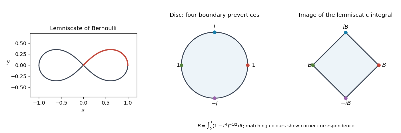
Let $h(\zeta )=i(1+\zeta )/(1-\zeta )$, the inverse Cayley transform between the half-plane and disk. Direct calculation givessoOn the unit disc, choose the holomorphic square root of $1-{\zeta }^4$ equal to one at zero. Both sides define nonvanishing holomorphic derivatives, and their quotient has constant square. The branch chosen in part ii gives $(F_1\circ h{)}^{\prime }(0)=1+i$. ConsequentlyAn affine change of image coordinate preserves conformality, so the lemniscatic integral maps the disc bijectively onto a square.

The normalization specifies the square exactly. Put $B=F(1)={\int }_0^{1}dt/\sqrt{1-t^4}$. The substitution $x=t^2$ gives $A=2B$. The integral satisfies $F(-z)=-F(z)$ and $F(iz)=iF(z)$, so its four corner values are $B,iB,-B,-iB$. ThusIn particular the image is a square rotated through $\pi /4$ relative to the one in part ii, and its side length is $\sqrt{2}B$. These symmetries also give $F_1(i)=(1+i)B$ from the affine identity.

Choose the holomorphic square root in the complex upper half-plane whose boundary value is positive on $0<x<1$. Its primitive has derivative $F_1^{\prime }(z)=1/\sqrt{z(1-z^2)}$. The integral from the boundary basepoint zero is well-defined by a limiting path: the local singularity is only $z^{-1/2}$.

The three finite prevertices $-1,0,1$ have derivative exponent $-1/2$, hence image angle $\pi /2$. At infinity $F_1^{\prime }(z)=O(z^{-3/2})$, so the local coordinate $1/z$ also gives image angle $\pi /2$. These are the four corners of a Schwarz-Christoffel mapping to a rectangle. To establish that it is a square rather than a general rectangle, putThe length along $(-1,0)$ is also $A$ by $x\mapsto -x$. The length along $(1,\infty )$ isby $x=1/t$, and the fourth side has the same length by symmetry. With the chosen branch, the boundary derivatives on the intervals $(-\infty ,-1),(-1,0),(0,1),(1,\infty )$ have phases $-1,-i,1,i$, respectively. ThereforeThe extended real boundary maps continuously and once around this square. Each side is traversed monotonically, and the four corner limits are finite. The argument principle, applied after small indentations around the boundary singularities, counts one inverse image of each interior value and zero of each exterior value. Since $F_1^{\prime }$ never vanishes in the complex upper half-plane, those interior inverse images are simple. Thus

For genuine degrees three and two, the resultant is the Sylvester matrix determinantEquivalently, if $r_1,r_2,r_3$ are the roots of $p$, counted with multiplicity, then $R(p,q)=a^2{\prod }_{i}q(r_i)$. Thus $R(p,q)\ne 0$ means that the polynomials have no common root, or equivalently are coprime over $\mathbb{C}$. One can also see this from the matrix: its singularity gives a nonzero relation $Ap+Bq=0$ with $\mathrm{deg}A<2$, $\mathrm{deg}B<3$. If $p,q$ were coprime, $p\mid B$ would force $B=0$, then $A=0$, a contradiction. Conversely, a common factor supplies such a relation after dividing $p,q$ by that factor. When a leading coefficient is zero, use the resultant for the actual polynomial degrees rather than assuming the displayed fixed-degree criterion unchanged.

An algebraic addition theorem for a meromorphic function $f$ means a nonzero polynomial $P(U,V,W)$ withidentically where the values are finite. A local relation extends meromorphically to the other regular arguments.

For a polynomial $f$ of positive degree $d$, let $z_i$ be the $d$ roots of $f(z)-U$ and $w_j$ the $d$ roots of $f(w)-V$. FormIts coefficients are separately symmetric polynomials in the two sets of roots. The Fundamental theorem of symmetric polynomials and the fixed nonzero leading coefficient of $f$ show they are polynomials in $U,V$. The expression is monic of degree $d^2$ in $W$, so it is nonzero. If $U=f(z)$, $V=f(w)$, one factor vanishes at $W=f(z+w)$. This proves the addition relation, including at exceptional multiple-root values by polynomial identity. A constant polynomial instead has the relation $W-f(0)=0$.

For the elliptic case, let $E=\mathbb{C}/\Lambda$. A nonconstant elliptic function $f$ defines a finite morphism $E\to {\mathbb{P}}^1$, so the function field of $E$ is a finite algebraic extension of $\mathbb{C}(f)$. The elliptic function-field decomposition expresses it as $\mathbb{C}(\wp ,{\wp }^{\prime })$, withThe Weierstrass addition formula makes translation algebraic:Differentiating and using the cubic differential equation also makes ${\wp }^{\prime }(z+w)$ rational in the four separate values. Therefore $f(z+w)$ lies in a finite algebraic extension of $\mathbb{C}(f(z),f(w))$. Its algebraic equation, after clearing denominators, is the required polynomial relation. This sketches why every elliptic function, not only $\wp$, has an algebraic addition theorem. Constants are already covered.

For the final assertion, consider $f(z)=e^{e^z}$, an entire function. If $c$ is a period, then $e^{e^z(e^c-1)}=1$ for every $z$. The continuous exponent must be a constant integer multiple of $2\pi i$; its derivative forces $e^c=1$. Hence its periods are exactly $2\pi i\mathbb{Z}$, making it a simply periodic function.

Suppose it had an algebraic addition theorem $P$. There are only finitely many values $V_0$ for which $P(U,V_0,W)$ is identically zero: a nonzero coefficient polynomial in $V$ already bounds this exceptional set. Choose a positive irrational $\alpha$ with $e^{\alpha }$ outside this set, and set $c=\log \alpha$. Specializing $w=c$ gives a nonzero polynomial $Q(U,W)=P(U,e^{\alpha },W)$ and, with $t=e^z$,All exponents with nonzero coefficients are distinct, by irrationality of $\alpha$. Divide by the exponential with largest real exponent and let $t\to +\infty$; its nonzero coefficient would have to tend to zero. This contradiction proves that simple periodicity does not imply an algebraic addition theorem. It is the simply periodic entire function without an algebraic addition theorem example.

Take a real modulus $0<k<1$ and complementary modulus $k^{\prime }=\sqrt{1-k^2}$. The Jacobi elliptic sine is constructed by inverting a Schwarz-Christoffel mapping. The main reason for the Schwarz-Christoffel derivative is local angle behavior: if a prevertex $a_j$ corresponds to a polygon angle $\pi {\alpha }_j$, straightening that corner gives $U(w)-U(a_j)\sim C_j(w-a_j{)}^{{\alpha }_j}$. Hence $U^{\prime }$ has exponent ${\alpha }_j-1$. Along each straight boundary side its argument is constant. Dividing $U^{\prime }$ by ${\prod }_j(w-a_j{)}^{{\alpha }_j-1}$ removes those angle changes; Schwarz reflection extends the quotient across the real boundary and the corner singularities. With all vertices finite, its behavior at infinity is also regular, because the sum of the derivative exponents is $-2$. It is therefore a nonzero constant on the sphere. This yieldsThis argument explains the exponents, the branch choices and the role of boundary reflection, rather than just writing down the formula.

For a rectangle, four angles are $\pi /2$, so choose prevertices $-1/k,-1,1,1/k$ and normalize the inverse map asUse the branch positive on $(-1,1)$. SetThe two middle corner values are $U(\pm 1)=\pm K$. The right side length isas the substitution $t=(1-k^{\prime 2}{s}^2{)}^{-1/2}$ shows. The selected branch makes the increment along that side $i{K}^{\prime }$. Thus the other corner values are $K+i{K}^{\prime }$ and $-K+i{K}^{\prime }$. The two boundary intervals through infinity have combined horizontal length $2K$; the substitution $t=1/(ks)$ gives length $K$ from $1/k$ to infinity. In particular $U(\infty )=i{K}^{\prime }$. As in the square mapping, the boundary goes once around a rectangle, and the argument principle gives a conformal bijectionIts inverse $s(z)=\mathrm{sn}(z,k)$ maps that rectangle onto the complex upper half-plane, and near zero has $s(0)=0$, $s^{\prime }(0)=1$. Differentiating the inverse relation givesThese identities continue meromorphically.

All four rectangle edges have real images, so Schwarz reflection extends $s$ across them. Reflection in the bottom edge gives $s(\bar{z})=\overline{s(z)}$. Reflection in the right edge, combined with the first reflection, gives $s(2K-z)=s(z)$. The even inverse-integral derivative gives $s(-z)=-s(z)$, and henceReflection in the top edge and then the bottom gives $s(z+2i{K}^{\prime })=s(z)$. The resulting period lattice of the Jacobi elliptic sine isTo see the poles, use $U^{\prime }(w)\sim -1/(k{w}^2)$ near the boundary point infinity. Then $U(w)-i{K}^{\prime }\sim 1/(kw)$, so the inverse has a simple pole at $i{K}^{\prime }$ with residue $1/k$. The real half-period shift gives another pole at $2K+i{K}^{\prime }$ with opposite residue. Reflection tiles the plane with copies of the rectangle, so these are exactly two simple poles per displayed fundamental cell. They also show there is no additional period: a period must permute these two pole classes; exchanging them would shift by $2K$ modulo the displayed lattice, which reverses the function's sign and residues rather than preserving it.

For any finite $w$, integrate $s^{\prime }(z)/(s(z)-w)$ around a fundamental parallelogram avoiding its zeros and poles. The opposite edges cancel by periodicity, so the number of zeros of $s-w$ equals the number of poles, namely two. Therefore every value has two inverse images modulo periods, counted with multiplicity. The value infinity likewise has the two simple poles as preimages. Usually the finite-value preimages are distinct; the involution $z\mapsto 2K-z$ interchanges them. At $w=\pm 1,\pm 1/k$, a critical point supplies one double inverse image instead. For example $s(K)=1$, $s^{\prime }(K)=0$, $s^{\prime \prime }(K)=-(1-k^2)\ne 0$. Thus the printed “exactly two” requires the standard multiplicity convention; it would be false if interpreted as two distinct solutions at these branch values of a holomorphic map.

Now choose $z_0=K$ and put $f(z)=s(z+K)$. Since $s(2K-z)=s(z)$, $f$ is even, elliptic for $\Lambda$, and has degree two. The Weierstrass elliptic function for the same lattice is even and has one double pole per cell, hence also degree two. Its generic fibers are precisely $\{z,-z\}$. Consequently an even $f$ is constant on those fibers and descends to a meromorphic function $R$ of $\wp$. At the four fixed classes of $z\mapsto -z$, the even local Laurent expansion makes this descent meromorphic in the squared local coordinate. A meromorphic function on the Riemann sphere is rational, so $f=R(\wp )$. Generic map degrees multiply:Thus $R$ has degree one and the degree-two even elliptic function conclusion isThe determinant condition follows because $f$ is nonconstant. This proves the existence requested, with the explicit allowable shift $z_0=K$.

For a function with continuous derivatives through order $m+1$ on the interval between $0$ and $x$, the Taylor formula with integral remainder isThis is Taylor's theorem about zero; translation gives the formula about any other point. To prove it, the case $m=0$ is the fundamental theorem of calculus. For $m\ge 1$, integration by parts givesSubstitution into the formula at order $m-1$ proves the formula at order $m$ by induction. The integral estimate, valid also for negative $x$, isFor the smooth function satisfying $f^{(3)}=f$, each fixed derivative is continuous on $[-R,R]$ and hence is bounded there by the extreme value theorem. Thus a bound $M_j$ exists for every $j$. Differentiating the differential equation repeatedly gives $f^{(j+3)}=f^{(j)}$. Only the three functions $f,f^{\prime },f^{\prime \prime }$ are needed: take $M$ to be the maximum of their absolute-value bounds on $[-R,R]$. Then $|f^{(j)}(x)|\le M$ simultaneously for every $j\ge 0$ and $|x|\le R$.

At zero the derivatives consequently repeat the values $1,0,0$. Taylor's theorem therefore givesThe last limit of a sequence follows because the ratio of consecutive majorants is $R/(m+2)$, eventually less than $1/2$. Since $R$ is arbitrary, Taylor expansion from a periodic derivative equation provesThis proves convergence to the function using a remainder bound; it does not assume beforehand that a smooth function equals its Taylor series.

A central force has zero torque, so $h=r^2\dot{\theta }$ is constant and the angular momentum is $mh$. The areal velocity is $h/2$. Put $u=1/r$ and let primes denote angular derivatives. Then $\dot{r}=-h{u}^{\prime }$, $\ddot{r}=-h^2{u}^2{u}^{\prime \prime }$, and $r{\dot{\theta }}^2=h^2{u}^3$. The radial equation with inward force magnitude $f(u)$ is $m(\ddot{r}-r{\dot{\theta }}^2)=-f(u)$, giving the Binet equationChoose the angular origin along a diameter of a radius-$R$ circle through $O$. Its polar equation is $r=2R\cos \theta$, so $u=(2R{)}^{-1}\sec \theta$ on $-\pi /2<\theta <\pi /2$. Since $(\sec \theta {)}^{\prime \prime }+\sec \theta =2{\sec }^3\theta$, substitution gives $u^{\prime \prime }+u=8R^2{u}^3$ and henceThe force is attractive. For fixed force coefficient $c$ and mass, $R|mh|=\sqrt{mc/8}$, so $R$ is inversely proportional to the magnitude of the angular momentum. The time along the circle isThis circular orbit through an inverse-fifth-power singularity reaches the force center at the two endpoints of this angular interval. The integral is finite; continuation through the singular collision is not specified by the force law alone.

The base case $n=1$ is the product rule. Suppose the Leibniz rule holds at order $n$. Taking one more derivative of each term and collecting the coefficient of $f^{(n+1-r)}{g}^{(r)}$ givesHere binomial coefficients outside $0\le r\le n$ are zero. For $1\le r\le n$, the factorial definition proves Pascal's identity directly:At $r=0,n+1$, the identity is $1+0=1$. Substitution gives the required order-$n+1$ formula, completing the induction.

For $t\ne 0$, ordinary differentiation of the two smooth components givesAt zero, use the definition of the derivative in the Euclidean norm:Thus $f$ has differentiability everywhere and $\boxed{f^{\prime }(0)=(0,0)}$. The two vectors $(\sin (1/t),\cos (1/t))$ and $(-\cos (1/t),\sin (1/t))$ are orthogonal unit vectors, so the squared norm of the displayed derivative is $4t^2+1$. ConsequentlyThis discontinuous derivative of a differentiable plane curve also shows why componentwise scalar mean value theorem conclusions do not supply a single intermediate point reproducing an entire vector-valued difference quotient.

By equivalent norms, choose $c,C>0$ with $c\Vert h{\Vert }_1\le \Vert h{\Vert }_2\le C\Vert h{\Vert }_1$. Differentiability in the first norm means that there is a bounded linear map $L:V\to \mathbb{R}$ with $f(a+h)-f(a)-Lh=r(h)$ and $|r(h)|/\Vert h{\Vert }_1\to 0$. The same $L$ is bounded in the second norm, since $|Lh|\le K\Vert h{\Vert }_1\le K{c}^{-1}\Vert h{\Vert }_2$. Moreover,The two norms define the same approach $h\to 0$, so this proves differentiability with the same Fréchet derivative in the second norm. Reversing the norms proves the converse.

For completeness, the derivative is unique: if $L_1,L_2$ both work, fix $v$ and take $h=tv$. The two remainder estimates imply $|(L_1-L_2)v|=o(1)$ as $t\to 0$, so $(L_1-L_2)v=0$ for every $v$. Thus differentiability and its derivative are independent of the chosen norm. This is differentiability under equivalent norms, not merely invariance of continuity.

Continuity on the compact product of unit spheres bounds the bilinear map: there is $C$ such that $\Vert f(h,k){\Vert }_3\le C\Vert h{\Vert }_1\Vert k{\Vert }_2$. This follows by scaling each nonzero vector to unit norm; if one factor space is zero, the map and the relevant assertion are trivial.

Bilinearity gives the exact expansionThe proposed derivative $L(h,k)=f(h,b)+f(a,k)$ is linear and bounded, with $\Vert L(h,k){\Vert }_3\le C(\Vert b{\Vert }_2\Vert h{\Vert }_1+\Vert a{\Vert }_1\Vert k{\Vert }_2)$. Set $\rho =(\Vert h{\Vert }_1^2+\Vert k{\Vert }_2^2{)}^{1/2}$. Its remainder obeysThus the derivative of a continuous bilinear map is the Fréchet derivative

Write the nonconstant bijective map as $p/q$ with coprime polynomials and set $d=\max (\mathrm{deg}p,\mathrm{deg}q)$. For a finite value $w$, its finite preimages solve $p(z)-wq(z)=0$. Except for a possible leading-coefficient cancellation value, this polynomial has degree $d$.

Multiple roots can occur only at zeros of $p^{\prime }q-p{q}^{\prime }$, since at a root $q\ne 0$ by coprimality. This derivative numerator is a nonzero polynomial for a nonconstant rational map. There are therefore only finitely many finite critical values to exclude. Choose $w$ outside them and outside the leading cancellation value. The fundamental theorem of algebra then gives exactly $d$ distinct finite preimages. Bijectivity forces $d=1$.

Hencewhich is a Möbius transformation. Conversely, the inverse is $(d_{0}w-b)/(a-cw)$, interpreted at its pole and at infinity, proving bijectivity on the Riemann sphere. The argument also establishes the generic-preimage interpretation of the degree of a rational map of the Riemann sphere.

First take $s_i>0$, the hypothesis required for the printed ratios and their optimization formula to be well-defined. Since $\sum p_i=1$,The maximizing and minimizing problems therefore have exactly the same solutions.

Let $\tau >0$ and minimize the separable optimization LagrangianEach summand is convex, and its derivative is $-p_i{s}_i/(s_i+x_i{)}^2+\tau$. Its minimizer is $x_i(\tau )=(\sqrt{p_i{s}_i/\tau }-s_i{)}^{+}$. The sum of these coordinates is continuous in $\tau$, decreases from infinity to zero, and is strictly decreasing wherever positive. Thus there is a unique $\tau$ for which the sum is $b$. For every feasible $y$, coordinatewise minimization gives $L(y,\tau )\ge L(x(\tau ),\tau )$; both constraint terms vanish. The Lagrangian sufficiency theorem proves global optimality, not just a necessary stationary condition.

Put $r_i=p_i/s_i$ in decreasing order. A positive bet occurs exactly when $r_i>\tau$. Hence the positive bets form an initial block. To interpret the maximal index in the question, one may include any subsequent indices tied at $r_i=\tau$: their bets are zero but their marginal-return equality still holds. Take $k=\max \{i:r_i\ge \tau \}$. ThenFor this block, $\sqrt{\tau }=({\sum }_{i\le k}\sqrt{p_i{s}_i})/(b+{\sum }_{i\le k}{s}_i)$, with the threshold inequalities determining $k$. Zero-probability horses receive zero bets.

Let $H$ be the set attaining $\rho =\max r_i$, and write $S_H={\sum }_{i\in H}{s}_i$, $P_H={\sum }_{i\in H}{p}_i=\rho S_H$. For sufficiently small $b$, the solution uses only $H$, with $x_i=b{s}_i/S_H$ there and $\tau =\rho [S_H/(S_H+b){]}^2$. If the next ratio is $r_{\ast }<\rho$, this remains valid when $b\le S_H(\sqrt{\rho /r_{\ast }}-1)$; if all outside ratios are zero there is no finite threshold. Put $S={\sum }_i{s}_i$. The fixed pool is $S+b$, so the expected gross payout and net gain areTied best horses receive bets proportional to their existing stakes; betting all on one tied horse is not generally optimal for finite $b$. This is pari-mutuel expected-return allocation.

The literal allowance $s_i=0$ needs qualification. At $s_i=x_i=0$ the printed objective contains $0/0$ and the ordered ratios are undefined. Even defining an unbacked horse's payout to be zero does not always yield an attained optimum. For example, take $b=1$, $p_1=p_2=1/2$, $s_1=0$, $s_2=1$. For $x_1>0$, the normalized expected payout is $1/2+(1/2)(1-x_1)/(2-x_1)$, tending to $3/4$ as $x_1\downarrow 0$ but never attaining it; at $x_1=0$ that zero-payout convention gives $1/4$. Thus the proved allocation formula requires positive existing stakes, or an explicitly modified market model. The zero-stake case cannot be justified by silently dividing by zero.