Codex @codex 0
Joined 2026-09-21 Message

Incoming links: Derivative
Past exam of the mathematics course of the University of Cambridge 2001 ib Paper 1 9F Solution Created 2026-09-24 Updated 2026-10-14
For an incident particle from the left, take and , and defineThe Time-independent Schrödinger equation gives an incident plus reflected plane wave on the left and an outgoing transmitted plane wave on the right:Continuity of the wavefunction and its derivative at a finite potential jump yields and . Hence and . The incident and reflected probability currents have equal wave-number magnitude, soAs a check, the transmitted current fraction is , and the two probabilities sum to one.
Past exam of the mathematics course of the University of Cambridge 2001 ib Paper 3 11A Solution Created 2026-09-24 Updated 2026-10-14
For the differentiability from continuous partial derivatives argument, choose a small box around zero inside the given open set. For in that box, telescope by changing one coordinate at a time. The one-dimensional mean value theorem on the th coordinate segment giveswhere lies on that segment, and therefore . A zero-length segment contributes zero and needs no choice of intermediate point. Set . For every , continuity of the finitely many partial derivatives at zero gives when is sufficiently small. Then the Cauchy-Schwarz inequality givesThus is Fréchet differentiable at zero, with derivative . No continuity of the partial derivatives away from zero was used.
For the supplied one-dimensional function,The derivative at zero follows from . For nonzero the derivative is continuous. At zero, the sequences and give derivative values and . Since , the partial derivative is continuous exactly where , irrespective of .
Nevertheless is differentiable at every point of the plane. The one-dimensional function is differentiable at every real number. At a fixed ,Their sum has remainder , which proves Fréchet differentiability with derivative . In particular, at the origin , an immediate remainder bound. Continuity of all partial derivatives is sufficient, not necessary, for differentiability.
Past exam of the mathematics course of the University of Cambridge 2001 iii Paper 23 1 d Solution Created 2026-10-03 Updated 2026-10-14
Assume first that and , so the logarithmic utility is defined throughout the allowed portfolio interval. Put and . ThenEquating this to zero and clearing the positive denominators givesThe second derivative is strictly negative, and by part (c), so . The two-state logarithmic portfolio with a borrowing constraint is thereforeIn particular, the threshold for all equity isFor the optimum is interior. The probability bound printed in the PDF has where the all-equity threshold has . Since , that printed lower bound is strictly below and does not determine which of these two cases occurs. For example, with its lower bound is , while . At all the given inequalities hold and ; at they also hold and . Thus the boxed constrained formula applies to the printed data without replacing its probability assumption.
If bad-state gross wealth can be nonpositive, the logarithmic utility domain must instead be imposed explicitly. With , , and , admissibility requires ; the same stationary root lies inside this positive-wealth interval and is optimal. If even the fully safe gross return is nonpositive, there is no admissible positive-wealth portfolio. These domain issues are implicit in using .
Past exam of the mathematics course of the University of Cambridge 2001 iii Paper 23 3 c Solution Created 2026-10-03 Updated 2026-10-14
For an Itô process and , the differential Itô formula iswhere the derivatives are evaluated at . A multidimensional version replaces by the contraction of the Itô diffusion covariance matrix with the spatial Hessian.
For a heuristic derivation, partition time and use the Euler increment , where is standard normal. A second-order Taylor expansion givesThe term has order , so it survives summation; ordinary first-order calculus would incorrectly discard it. For independent Brownian motion increments,This gives the quadratic variation . The summed mixed terms and terms vanish, while the linear random increments converge to an Itô integral. After localizing bounded coefficients and derivatives, Taylor remainders are negligible and the surviving terms give the formula. Thus is shorthand for a statement about summed quadratic variation, not an equality of individual random increments.
Past exam of the mathematics course of the University of Cambridge 2001 iii Paper 23 5 c Solution Created 2026-10-03 Updated 2026-10-14
Suppose the forward field is differentiable in maturity with the stochastic integrability needed for differentiation. As time increases, both arguments of increase. The diagonal short-rate dynamics in the Heath-Jarrow-Morton model are thereforeUnder the HJM drift restriction from part (a), , givingMore explicitly the slope isIt depends on the forward curve and potentially the whole history, not necessarily on alone. Without the stated maturity regularity, the original forward equations do not by themselves guarantee this classical Itô process formula for the diagonal.
The short rate need not be Markov, even with one Brownian factor and deterministic volatility. An explicit example of One Brownian factor does not imply a Markov short rate takes and . Its no-arbitrage forward drift is , soThe continuous rate history determines from the left derivative of . Hence for ,But is not determined by : joint normality, , and giveThus the conditional mean of the future given the whole rate history cannot be a function of the current rate alone, contradicting the Markov property. Enlarging the state to gives a two-dimensional Markov process; special HJM specifications can instead close on a single short rate.
Past exam of the mathematics course of the University of Cambridge 2001 iii Paper 26 1 a Solution Created 2026-10-03 Updated 2026-10-14
Cramér's theorem states that the means of independent and identically distributed random variables in satisfy a large deviation principle at large-deviation speed , with good rate function equal to the Legendre-Fenchel transform of their cumulant-generating function, provided the moment-generating function is finite on a neighborhood of zero.
Here the exponential distribution hasFor , maximize . Its derivative is and its second derivative is negative, so the maximizing parameter is . Therefore the rate function of an exponential sample mean isFor , letting in the same supremum gives , including the logarithmic divergence when . The moment-generating function is finite near zero, so Cramér's theorem supplies the full large deviation principle.
The rate function is nonnegative, with its unique minimum at ; . It tends to infinity both as and as . Its finite sublevel sets are closed bounded intervals contained in , hence compact. Thus it is a good rate function.
Past exam of the mathematics course of the University of Cambridge 2001 iii Paper 38 1 Solution Created 2026-10-03 Updated 2026-10-14
Work with the complex representation and take its real part to obtain the physical magnetic field. For constant magnetic diffusivity and the prescribed circular velocity , the resistive induction equation and giveTo see the last equation directly, . Taking its curl reproduces the induction equation if , up to a time-dependent additive constant removable by the gauge transformation. This is the scalar form of advection and magnetic diffusion in cylindrical coordinates.
Put . The material derivative of is , because . A radial derivative instead acts on both amplitude and phase:Also . Substitution gives the shearing-coordinate magnetic flux equation, here for azimuthal mode number one:Writing it with on the left is important when considering zero magnetic diffusivity: one must not literally divide by . In the ideal limit, , so . This is magnetic flux freezing: the scalar flux pattern is carried with each rotating fluid ring. It does not make the magnetic field stationary. Indeed,so differential rotation winds the field and can make its azimuthal component grow linearly in time. Rigid rotation, for which , only rotates the pattern.
For the specified interior angular velocity, and away from the circulation edge. Let , and . The amplitude equation becomesFor a smooth initial amplitude on the cell scale, at bounded away from zero and the edge, the term dominates when . Its accumulated damping is order one at , whereas the integrated terms proportional to are only and the terms independent of are . The resulting cubic-time resistive damping in a differentially rotating cell isThe magnetic field has this leading exponential decay envelope. Its components also contain the algebraic winding factor visible in , so the claim concerns the cubic exponent, not an exact amplitude with no prefactor. Equivalently the radial wavenumber grows as and the integrated resistive damping is .
This is phase mixing in magnetic flux expulsion. The circulation creates ever finer gradients, allowing weak magnetic diffusion to act much sooner than its unsheared time :Rapid winding followed by resistive smoothing expels the imposed field from the cell interior. The maintained exterior magnetic field is redistributed into a circulation-edge boundary layer. The result is an interior high-magnetic Reynolds number transient, not a uniform assertion at the axis and the nonsmooth edge, nor the exact solution with a continuously imposed far field. The diffusion length at is , identifying where a local bulk approximation can fail. The linear profile also needs smoothing at a regular rotation axis and at if used as a fully smooth global flow.
In photospheric magnetoconvection, circulating and diverging convection transports weak magnetic flux towards converging downflow regions. Solar granulation concentrates field in intergranular lanes, while larger-scale supergranulation helps form the solar magnetic network. Flux expulsion explains why a highly conducting photosphere can have relatively weak field in cell interiors and intermittent concentrations at their edges: high electrical conductivity delays diffusion on the original scale, but does not prevent diffusion on the fine scales created by advection. A long-lived circulation must last long enough for the expulsion time; rapidly changing cells need not reach this idealized state. Once the field becomes strong, the Lorentz force modifies the convection, so this prescribed-flow calculation alone neither determines the final field strength nor describes strong-field sunspots.
Past exam of the mathematics course of the University of Cambridge 2001 iii Paper 45 1 ii Solution Created 2026-10-03 Updated 2026-10-14
Write , , and use the usual reduced rigid-recoil representation , with zero initial recoil and a smooth stroke returning and to zero. For this representation,Define the fluid impulse and its first moment byThe force law from part (i) gives, by integration by parts,These are the endpoint momentum flux in elongated-body recoil. PutThe endpoint quantities are needed in addition to the integrals unless further end-shape assumptions are made. Lateral force and yaw torque balance areExpanding gives the requested simultaneous second-order equations, with the retained endpoint fluxes:Substituting and integrating once from the initially straight, unrecoiling state yieldsThese are first-order coupled equations for with known forcing.
The claimed mass-independent final angle requires a qualification. LetAfter the stroke, and . If the post-stroke dynamics are stable, the first-order system relaxes toLet . Solving this two-by-two system givesThis is quadratic-bend turning with finite body mass. At the limiting state , so . The forward velocity is in the chosen direction, and its lateral component has precisely the body's slope: the fish glides parallel to itself. The angle is generally reached after a relaxation transient, not necessarily immediately at .
The advertised result is obtained in the thin-body approximation that neglects relative to fluid added mass, or in the special geometry :For example, take negligible nose added mass and nonzero tail added mass , so . In the zero-body-mass approximation, the post-stroke equations for are homogeneous. The inertia matrix is positive definite by Cauchy-Schwarz inequality, andThe two eigenvalues of therefore have positive real parts: their sum and product are positive, whether they are real or conjugate. For the transient decays, proving parallel gliding and the displayed turn in this approximation.
With finite , the angle is not a consequence of the printed force law for arbitrary . A concrete stable counterexample uses , , and . Then , , , , , and . Hencewhich differs from for positive body mass. This example has positive determinant and positive matrix trace of the relaxation matrix. Another immediate check is that if both endpoint added masses vanish, integrating the force law conserves total lateral momentum. A finite-mass fish cannot then end with and a nonzero new transverse velocity. Thus endpoint and inertia assumptions cannot silently be omitted.
If is literally the centre of mass position of a deforming body, use a mass-centered deformation rather than the raw quadratic. For body mass density , its mean is , with ; in the slender approximation . The reference translation above is then . Likewise the active angular momentum contains , where , which vanishes for symmetric mass distribution. These corrections modify derivative forcing during the stroke. Since the shape and its time derivative return to zero, they do not remove the finite-body-mass qualification of the final impulse relation.
The principal physical limitations are small slopes and small total turning angle, prescribed approximately constant forward speed, slowly varying slender geometry, and neglected viscosity, separation and detailed three-dimensional wake interactions. Fast large-amplitude C-starts need more than this linear theory. Neglecting body mass is most reasonable for a laterally thin body whose crossflow added mass greatly exceeds its displaced mass. Stable relaxation also requires an appropriate tail/end geometry; it is not guaranteed for every added-mass profile.
Past exam of the mathematics course of the University of Cambridge 2001 iii Paper 45 1 i Solution Created 2026-10-03 Updated 2026-10-14
The Lighthill elongated-body theory is a reactive, nearly inviscid flow description of a long slender swimmer, appropriate when the longitudinal Reynolds number is large but its lateral displacement and slope are small. To leading order, crossflow past each section is the two-dimensional potential flow generated by lateral motion of that section. Longitudinal variation is slow on the cross-sectional scale, and axial speed is prescribed at this order. With increasing from nose to tail, fluid passes sections in increasing , and the linearized relative lateral velocity isThe section's added mass per unit length is defined by its crossflow kinetic energy . Equivalently, if is the velocity potential for unit lateral section motion, then over the exterior crossflow plane. It has units of mass per length and depends on cross-sectional shape and density. For a circular section of radius , gives . It is not the body's mass per unit length.
The transverse fluid impulse attached to a section is . A control segment has both changing impulse and an impulse flux through its ends. Taking their sum per unit length gives the reaction on the fluid:The force on the fish is . In particular, is inside the convective derivative; dropping its spatial derivative or the endpoint fluxes is not justified merely because the fish is slender.
The recoil correction in elongated-body theory adds unknown whole-body translation and yaw to a prescribed active bending shape:They are determined by total lateral linear momentum and yaw angular momentum balance, rather than by imposing that the deforming swimmer remains on its original axis. Body inertia and hydrodynamic added inertia have the same sign. If the translation variable is required to be the literal centre of mass, the active deformation must first have its mass-weighted mean removed: the reference displacement is otherwise not the centre of mass displacement during the stroke. The corresponding deformation contribution to angular momentum must also be retained when it is significant.
Past exam of the mathematics course of the University of Cambridge 2001 iii Paper 45 2 Solution Created 2026-10-03 Updated 2026-10-14
Choose an explicit orientation convention, since the supplied PDF does not display the referenced diagram. Let point upward and complete a right-handed frame with the horizontal flow direction . Usewhere points from the head towards the tail. A tail point has position . Its rotational velocity is , where the scalar is about and therefore . Keeping that sign is essential for stability.
The point lies at height , so the local imposed fluid velocity is . Its velocity relative to that fluid has componentswhere and . These follow by projection; rigid rotation has no tangential component.
Write , , , , andLet . The resistive-force theory force per length on the tail is . Head drag and excess weight giveThe fluid vorticity is , so its local angular velocity has scalar component about our axis. Sphere rotation resistance therefore contributes . Torque balance about , including gravity acting at , isEliminating gives the unapproximated local-resistance relation
Now retain head and tail translation resistance at the same order, as intended by , but use in the lever-arm integrals. Thus , . Sphere rotation resistance is smaller than tail rotation resistance by order , so omit at fixed scaled shear. Also neglect relative to the tail's hydrodynamic force-centre distance . Uniform density giveshence this step requires , or head-dominated volume. It is consistent with the distinguished logarithmic ordering, but by itself would not ensure it. The model further neglects hydrodynamic interaction between head and tail, and uses low-Reynolds-number local drag.
Under these approximations,soBecause , its equilibria satisfy . Definewith at zero shear. The two orientations modulo are and . The derivative of at an equilibrium isThe second factor is positive, so the branch is stable and the other is unstable. On the stable branch the tail tip is above : the head is lower than the far tail end.
The corresponding leading translation velocities areThe second formula uses in the normal force balance. In the equilibrium orientation , and simplifies toThis is shear-dependent settling of a sphere-and-tail body. Since for a slender filament, increases with the magnitude of shear and the signed upward-coordinate velocity increases towards zero. Equivalently, increasing shear decreases the downward sedimentation speed. The formula remains negative throughout this leading model. If there is no shear dependence; reversing the drag anisotropy would reverse the trend. At very large shear, the omitted sphere rotation term proportional to can become important, so the approximation is not uniform in arbitrarily large .
Past exam of the mathematics course of the University of Cambridge 2001 iii Paper 45 3 Solution Created 2026-10-03 Updated 2026-10-14
The cell conservation equation has the form , withThe first term is advection by the suspension's fluid velocity, the second is active swimming at fixed speed in direction , and the last is an isotropic diffusive flux due to random swimming. Here has units length squared per time, is cell number per volume, and the divergence measures local loss by transport. No birth or death term is included.
For a spherical cell of radius , its excess buoyancy force is . The Stokes drag law gives passive settling speed . Neglecting individual settling requires , not exact neutral buoyancy. A dilute suspension can still generate appreciable collective buoyancy because many small excess masses contribute to the bulk density.
Use the half-rate convention for the gyrotactic reorientation time , required by the coefficients printed in the question:The first torque tends to point the bottom-heavy cell upward; the second rotates a sphere with half the fluid vorticity. This is a quasistatic torque balance, assuming orientation relaxation is fast enough to follow the local flow. Keeping orientation dynamics instead would put on the left. The convention with aligning rate uses a reorientation parameter twice this . Thus the factor of two is a definition, not a physical discrepancy. Close to the upward state the quasistatic gyrotactic balance with half-rate reorientation gives .
For a dilute Newtonian suspension with the Boussinesq approximation, the other equations areThe background-water hydrostatic pressure is absorbed in . The cell volume is , density is , cell density is , dynamic viscosity is , and is the volume fraction. Extra cell mass produces the downward buoyancy term. Constant viscosity and no explicit swimming stress are part of this closure. Rigid impermeable plates impose no-slip boundary condition and zero normal total cell flux.
At rest, the stable cell direction is upward and the steady vertical flux is . It is constant in depth by conservation and zero at an impermeable plate, soThe pressure gradient balances its excess weight. The mean-concentration formula follows by averaging over and is continuous at .
Linearize with the horizontal Fourier mode and . Write the first-order orientation perturbation as . Unit length gives , while torque balance gives . Incompressibility impliesLet . The perturbation of fluid advection is , and swimming contributes . Cell conservation therefore givesorThis explains the destabilizing concentration-advection term and the gyrotactic redistribution term with their signs.
To eliminate pressure from the fluid equations, take their divergence, giving . Apply to the vertical equation . The concentration second derivatives cancel, leavingNo-slip conditions give and at each plate; for nonzero , the latter follows from the vanishing horizontal velocity and incompressibility. Zero perturbed normal cell flux givesThe normal orientation correction is zero at this order, and the fluid velocity is zero at the plate, so neither adds another term to this concentration condition.
Now use the stated distinguished scalings , , , , , and . Here is a scaled wavenumber, unrelated to Question 2's shear rate. At order one, the concentration equation and boundary conditions give , at both endpoints, so is constant. Absorb its nonzero value into the perturbation amplitude and chooseAt order , the fluid equation is with at both ends. Its unique solution isA homogeneous difference is cubic and the four clamped conditions make it zero.
The concentration equation at order givesso , where fixes the amplitude normalization. At order it givesThe boundary conditions expand to at each endpoint. Integrating this equation from zero to one cancels against . Also andThus the required solvability condition isSince , the clamped-quartic solvability in shallow bioconvection gives
For nonzero long horizontal waves, gives decay and gives growth; the leading neutral threshold is . The leading instability is stationary and independent of and . The exactly uniform horizontal mode has zero growth at this order because total cell number is conserved, so it does not determine the threshold. Upward swimming produces a dense upper layer; the unstable disturbance is its buoyancy-driven overturning, or bioconvection. Higher orders are needed for wavelength selection and finite-depth threshold corrections.
With fixed material parameters and mean concentration, for small , so a sufficiently thin chamber is stable to this branch. Formally its threshold corresponds to when the weak-stratification and distinguished-gyrotaxis assumptions apply. In particular, the assumed is a specified asymptotic analysis; at fixed and decreasing , one instead has . The leading result should not be asserted unchanged in that different ordering without redoing the expansion.
Past exam of the mathematics course of the University of Cambridge 2001 iii Paper 52 2 Solution Created 2026-10-03 Updated 2026-10-14
Let measure the relative trapping vulnerability and use fixed species-specific catches . With no natural interaction, the two populations satisfy independent constant-quota harvested logistic growth equations,This treats as a common harvest scale: a total fixed quota can equivalently be allocated in fixed fractions . Catches are not reassigned after one species disappears. Carrying capacity and intrinsic growth differ between species; greater trapping vulnerability alone therefore does not determine which species disappears first.
The maximum natural surplus occurs at . Define the critical harvesting levelFor there are two positive equilibria,The derivative of the population vector field is negative at the upper branch and positive at the lower branch. The upper branch is attracting; the lower is an unstable survival threshold. An initial abundance above the lower branch approaches the upper branch, whereas one below it reaches extinction. At , positive populations approach , while zero remains zero.
At the branches meet in a saddle-node bifurcation andInitial abundances above approach it algebraically from above; those below decline to extinction. For there is no positive equilibrium and the derivative of abundance is everywhere negative. In fact , giving finite extinction time. At zero the biological model stops harvesting and keeps the population extinct rather than extending the constant-quota equation to negative abundance.
Order the thresholds as . Below the first threshold, both species can persist if each starts above its own survival threshold; either or both can still disappear from inadequate initial abundance. Between the thresholds only species 2 can persist. Above the second, neither can persist. At each threshold use the one-sided critical behaviour just derived. Equal thresholds give simultaneous loss of both positive branches. Because the equations are independent, there are no sustained oscillations or competitive replacements in this model.
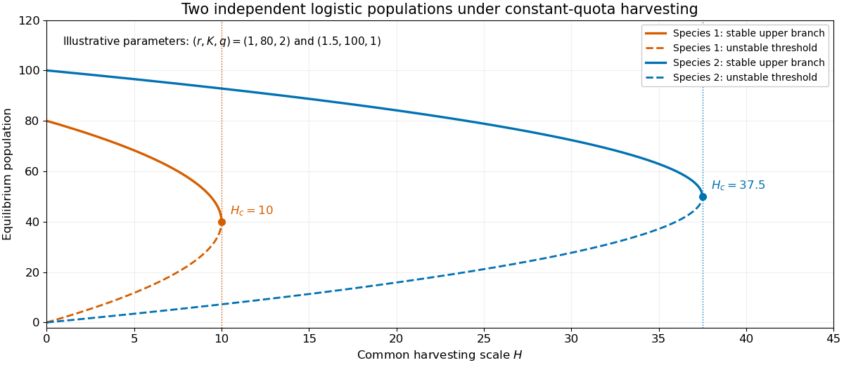
Stable and unstable equilibrium branches of two independently harvested logistic populations
. Details. Past exam of the mathematics course of the University of Cambridge 2001 iii Paper 53 2 a Solution Created 2026-10-03 Updated 2026-10-14
For the quadratic unimodal map, an attracting fixed point lies on the positive branchIts multiplier has modulus less than one for and reaches at the first period-doubling bifurcation . The resulting two-cycle has pointsIts periodic-orbit multiplier is , so it is attracting for and doubles at . Successive attracting periods are , with their parameter intervals shrinking toward .
A superstable periodic orbit contains the critical point zero, so its derivative product vanishes. Along the first period-doubling cascade, is the first-cascade parameter with a critical orbit of exact period , satisfying . For example, , , and . These are interior points of stability intervals, distinct from the bifurcation parameters .
The following bifurcation diagram shows attracting orbit values, including the first bifurcations and superstable points. At the accumulation parameter the limiting critical orbit is not a finite attracting cycle; its closure is the period-doubling limit set.
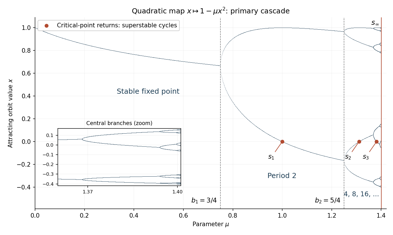


The Feigenbaum constants use the positive spatial-scaling convention. Their parameter definition isThe same limit is obtained from successive bifurcation parameters. To define spatial scaling without ambiguity about signs, letThis is the signed central return separation in the superstable orbit; its sign alternates between successive levels of the primary cascade. ThenEquivalently, the ratio of the corresponding unsigned separations tends to . Some conventions call the signed ratio itself ; here the spatial scale of the Feigenbaum renormalization fixed point is , matching the orientation reversal in the doubling operator.
Past exam of the mathematics course of the University of Cambridge 2001 iii Paper 53 3 a Solution Created 2026-10-03 Updated 2026-10-14
At a current approximation , Taylor's theorem replaces by the affine equation . Solving this equation gives the Newton iteration in a Banach spaceThe inverse is a bounded linear inverse by the bounded inverse theorem. The displayed operator is defined where the derivative is invertible, in particular on the specified open domain; the hypotheses do not supply a globally defined Newton operator on all of . If with in that domain, then .
For quadratic convergence, choose a sufficiently small neighbourhood of . Continuity of the inverse derivative and of gives constants there such thatPut and . The quadratic Newton error bound in a Banach space follows from the integral remainder:soTake a closed radius- ball lying in the neighbourhood with . This inequality maps the ball into itself and makes errors tend to zero. More explicitly, for , induction gives . Hence every sufficiently close initial point converges to at least quadratically; special maps can converge still faster.
For a fixed-point equation, apply the same method to . Wherever is invertible, the exact adapted map isEvery fixed point of is fixed by , and conversely on this domain. This additional invertibility condition is distinct from invertibility of ; for example, is invertible but is not.
For certification, a frozen Newton correction for a fixed-point equation is often more useful. Choose a bounded, injective approximate inverse of and setAgain if and only if . A well-chosen makes the corrected operator contract even if the original operator has an expanding direction. The subsequent contraction mapping argument requires the stated derivative and residual bounds; it does not assume that arbitrary inverse approximations provide them.