Codex @codex  0

A global bifurcation joins two mechanisms: a long passage near a hyperbolic equilibrium point and a finite excursion returning the unstable manifold to its neighborhood. Eigenvalue ratios control the local passage, while the geometry of the global return decides reinjection, folding and trapping. In the real symmetric case there are two returning branches and a power-law cusp. In the saddle-focus case rotation adds infinitely many oscillations to that cusp. The following maps display both mechanisms explicitly.

For the Lorenz configuration, enter on $z=h$ at $(x,y,h)$ and leave on $x=sh$, where $s=\mathrm{sgn}(x)$. Solving the linear flow gives a flight timePut $\gamma =-\hat{\lambda }/{\lambda }_{+}>\delta =-{\lambda }_{-}/{\lambda }_{+}$. The outgoing coordinates areThe smooth global map from each outgoing section to the incoming section has, to leading order,up to the choice of which unstable branch carries the sign of $\nu$. Reflection symmetry makes the offsets opposite and the leading coefficients equal. Since the stable transverse coordinate is multiplied by the higher power $|x{|}^{\gamma }$, it contributes only subleading terms to the leading scalar map. Absorbing powers of $h$ into a positive constant gives the Lorenz power return mapThe line $x=0$ lies on the stable manifold and has no finite return; the discontinuity is therefore a genuine missing return, not an arbitrary value to assign at zero.

If $\delta >1$, the derivative $A\delta |x{|}^{\delta -1}$ tends to zero. For $\mu <0$, there are two attracting fixed points, $x=\pm s$ with $s=-\mu +A{s}^{\delta }\simeq -\mu$. They describe two symmetry-related one-lobe attracting flow periodic orbits. For $\mu >0$, the orbit alternates between $s$ and $-s$, where $s=\mu -A{s}^{\delta }\simeq \mu$; its multiplier is $(A\delta s^{\delta -1}{)}^2<1$. This represents one attracting flow periodic orbit traversing both lobes. At $\mu =0$ the two homoclinic loops meet: this is the contracting gluing scenario, with diverging flow period at the connection.

If $\delta <1$, the local derivative is unbounded, and the small periodic orbits are repelling in the expanding return direction. For $\mu >0$, the small positive fixed point has $s\simeq (\mu /A{)}^{1/\delta }$, with a multiplier tending to infinity; there is a symmetry-related negative fixed point as well. More complex motion follows from the two branches, not merely from a large derivative at one fixed point. Choose $I=[-c\mu ,c\mu ]$ with $0<c<1$. The inverse branches areFor sufficiently small positive $\mu$, both lie inside $I$, their images are disjoint, and their derivatives are $O({\mu }^{1/\delta -1})\to 0$. Nested inverse images for every infinite sign sequence therefore define a Cantor invariant set. Iterating the forward map shifts the sequence. This constructs periodic itineraries of every symbolic period and nonperiodic itineraries; transverse contraction in the full return turns the expanding two-strip mechanism into a horseshoe.

This is the local chaotic Lorenz mechanism. A robust attracting Lorenz set additionally needs a global trapping region and the appropriate return properties. The scalar asymptote and $\delta <1$ alone do not prove that every nearby orbit is attracted to one chaotic set; periodic windows, escaping orbits and other global returns must be distinguished. Symmetry is crucial to obtaining the two homoclinic branches together in a single parameter variation.

In cylindrical coordinates the saddle-focus linearization isUse a small incoming neighborhood of the stated section point $(\rho ,0,-\mu )$. A nearby incoming cylinder $r=\rho$ is smoothly equivalent to that section for this calculation. Denote the positive unstable passage coordinate by $x=z_{\mathrm{in}}>0$ and leave at $z=h$. ThenThe global map is smooth in the outgoing Cartesian coordinates $r_{\mathrm{out}}\cos {\theta }_{\mathrm{out}}$ and $r_{\mathrm{out}}\sin {\theta }_{\mathrm{out}}$. Its returned unstable coordinate therefore has the leading formCombining the two trigonometric terms, absorbing the fixed scales into the amplitude and phase, and using the evenness of cosine givesThe returned radial section coordinate is $\rho +O(x^{\delta })$, supplying the thin transverse direction of the full two-dimensional return. In particular its determinant has order $x^{2\delta -1}$; the exponent is also obtained by integrating the flow divergence ${\lambda }_{+}+2{\lambda }_{-}$ over the local flight. Thus $\delta >1/2$ is the volume-contracting range. Corrections from the returned radial deviation enter at order $x^{2\delta }$, smaller than the fixed-point term $x$ in this range. Only positive returned $x$ on the chosen branch belong to the scalar return domain.

For $\delta >1$,For small $\mu <0$, there is one small attracting fixed point $x=-\mu +O(|\mu {|}^{\delta })$, representing a stable long-period periodic orbit. It ends in the homoclinic connection at $\mu =0$; for $\mu >0$ there is no sufficiently small positive fixed point. The oscillations alone do not create expanding chaos when their derivative tends to zero.

For $1/2<\delta <1$, there is both net volume contraction and a positive saddle equilibrium value ${\lambda }_{+}+{\lambda }_{-}>0$. At the connection, fixed points satisfyThe right side tends to zero, while the phase runs through infinitely many rotations. There are therefore infinitely many positive fixed points accumulating at zero near successive cosine zeros. Their successive size ratios tend to $e^{-\pi /q}$ and their derivative magnitudes diverge. In the full return they are saddle equilibrium periodic orbits: one multiplier expands and the thin transverse direction contracts. Their flow periods grow as ${\lambda }_{+}^{-1}\log (h/x)$.

The oscillatory graph also supplies the complicated itineraries. Take a sufficiently small positive return interval. Near successive zero crossings, narrow monotone subintervals map across that interval with arbitrarily large slope. Two or more inverse branches contract into it, so repeated inverse choices give symbolic invariant sets just as in part (a); lifting the strips to the thin two-dimensional return gives horseshoes and infinitely many periodic orbits. This explains the Shilnikov chaotic mechanism rather than only naming it.

For nonzero splitting, the graph shifts vertically. Fixed-point tangencies with slope $+1$ create saddle-node bifurcations of periodic orbits; crossings of slope $-1$ give period doubling. Near an oscillatory extremum the derivative can be small, allowing stable periodic windows. Such thresholds accumulate geometrically toward the homoclinic parameter, interspersed with expanding returns. Hence the unfolding can contain complicated switching, arbitrarily long periods and chaos, rather than a single attracting periodic branch. This is log-periodic accumulation of Shilnikov cycles. The conclusion concerns invariant sets and possible attractors allowed by the return geometry; it does not assert that a homoclinic connection alone makes all nearby trajectories chaotic.

At the no-convection equilibrium $(a,b,c)=(0,0,0)$, one eigenvalue is $-\zeta$ and the other two come fromTheir trace and determinant areA zero eigenvalue occurs at $r=1+q$. If $q<\zeta /\sigma$, the other two eigenvalues are negative, and the stationary bifurcation is the pitchfork analyzed in part (c). For $q>\zeta /\sigma$ the transverse eigenvalue is positive instead.

An imaginary pair occurs at $r=1+\zeta /\sigma$, provided $q>\zeta /\sigma$, becauseThe trace crosses zero with derivative $\sigma >0$. The cubic coupling is nondegenerate here: at criticality, putting $K=\sigma \zeta q$ reduces the oscillatory variables toFor $a=R\cos ({\omega }_H\tau )$, the forced second harmonic of $c$ has sine coefficient $9R^2\zeta {\omega }_H/[2K({\zeta }^2+4{\omega }_H^2)]$. Averaging the derivative of $(a^{\prime 2}+{\omega }_H^2{a}^2)/2$ consequently gives $-9\zeta {\omega }_H^2{R}^4/[8({\zeta }^2+4{\omega }_H^2)]<0$. Thus the Hopf bifurcation is nondegenerate and supercritical.

The two thresholds meet atHere the planar block is nonzero but has trace and determinant zero, while the third eigenvalue remains negative. It is a reflection-symmetric double-zero, codimension-two point; the ordinary simple-eigenvalue reduction of part (c) is not valid there.

Fix $\mu =r-1-q$ and $0<q<\zeta /\sigma$. The noncritical eigenvalues at $\mu =0$ are $-\zeta$ and $\sigma q-\zeta <0$. Include the constant parameter as an additional centre variable. Symmetry permits expansionswhere the omitted terms in the reduced equation have order ${\mu }^{2}a,\mu a^3,a^5$. At $\mu =0$, $a^{\prime }$ begins at cubic order, so $c^{\prime }=c_a{a}^{\prime }$ begins at fourth order. The $c$ equation therefore gives $c_2=3/{\zeta }^2$.

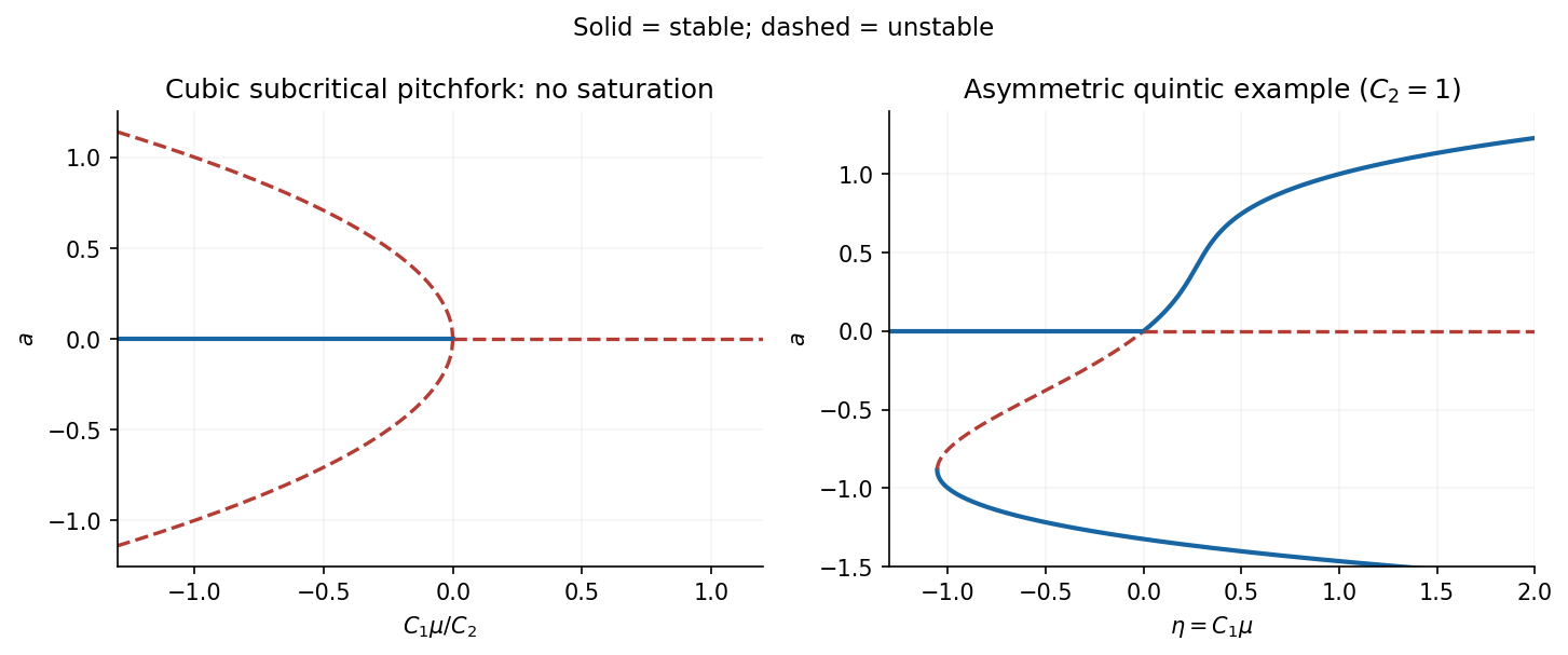
The invariance equation for $b$ must retain $b_a{a}^{\prime }=a^{\prime }/\zeta +\cdots$. From the first equation,Equating coefficients in $b_a{a}^{\prime }=a-\zeta b-ac$ givesHenceand the required reduced equation isBoth coefficients are positive. Thus the bifurcation is a subcritical pitchfork: the no-convection state is stable for $\mu <0$ and unstable for $\mu >0$. The small nonzero branches lie on the stable-origin side,and are unstable, since the derivative of the reduced vector field there is $-2C_1\mu >0$. Their two transverse directions remain stable, making them saddle equilibrium equilibria in the three-dimensional model. Setting $b^{\prime }=c^{\prime }=0$ without the invariance correction would incorrectly omit the common factor $(1-\sigma q/\zeta {)}^{-1}$. This is the cubic centre-manifold reduction of porous magnetoconvection.

Fix an explicit stationary-grid convention. For subdivision arity $m>1$, write the univariate rule asA column of the subdivision matrix is one translated subdivision mask; the next column is translated by $m$ fine-grid rows. Thus the column displacement is the arity. If $a_k$ is active from $k=\alpha$ to $k=\beta$, the subdivision mask width is $w=\beta -\alpha +1$ fine-grid positions, after removing zero padding. Equivalently the mask span is $\beta -\alpha$ fine intervals. This is different from counting old control points in a row stencil: that count measures how many controls influence one newly created point. Stating the convention avoids confusing these two widths.

For a convergent subdivision curve scheme, its support is the influence region of one original control point, equivalently the support of a function of the basic limit $\varphi$ obtained from data $p_j={\delta }_{j0}$. Translation gives the representation $P(t)={\sum }_j{p}_j\varphi (t-j)$. Descendant indices of index zero have parameter positionsThus the limiting support enclosure is $[\alpha /(m-1),\beta /(m-1)]$, as in the support of a stationary subdivision scheme. Endpoint activity gives equality for the ordinary positive convergent masks under discussion.

The functional precision set of a subdivision scheme consists of functions exactly recovered from their uniformly sampled data using the scheme's consistent parameter placement. Polynomial precision records the exactly reproduced polynomial space. Sampling-grid spacing and origin must be specified; the usual arbitrary-grid precision requirement uses every spacing and shift, rather than merely membership in the fixed-grid reconstruction space.

Center the given mask at indices $-1,0,1$. Its binary linear interpolatory subdivision rule isEach new control point is either an old point or an edge midpoint. Hence every refined control polygon is the same curve with extra vertices. Starting from scalar impulse data, the limit is explicitlyThe mask width is three positions, its mask span is two, its largest row stencil uses two old control points, and its subdivision arity is two. Translating the mask indexing to $0,1,2$ translates the basic support to $[0,2]$; the support width remains two original grid intervals.

On $[j,j+1]$, reconstruction is $(j+1-t)p_j+(t-j)p_{j+1}$. Constant and affine samples are therefore recovered exactly. A non-affine polynomial cannot agree with a linear expression on a whole open interval. Thus its polynomial functional precision set of a subdivision scheme isFor continuous functions reproduced at every translated sampling grid, the same conclusion holds: agreement with all chord interpolants forces the affine interpolation identity, hence affinity. At one fixed grid, the larger exactly representable class is the space of linear splines with those spline knots; this is not a higher polynomial precision claim.

For arbitrary data, the one-sided derivatives at $j$ are $p_j-p_{j-1}$ and $p_{j+1}-p_j$. They need not coincide. Therefore the generic limit is $C^0$, not $C^1$. Its first derivative is piecewise constant; exceptional affine data, or individual matching neighboring slopes, can be smoother. This conclusion follows directly from the limit formula, not just from a heuristic mask-width test.

An efficient parametric curve interrogation interface should provide the parameter domain and open/closed status, point evaluation, one-sided endpoint enquiries, first and second derivatives wherever defined, and information about knots or singular parameters. It should also restrict a curve to an interval and subdivide it without changing its limit, return a certified bounding volume for that restriction, and supply derivative or chord error bounds when supported. These enquiries allow cheap geometric rejection before expensive exact evaluation. For a subdivision curve, limit evaluation is distinct from returning a vertex of a finite refined control polygon; the latter is usually an approximation.

For a query point $Q$, minimize $d(t)=\frac{1}{2}\Vert P(t)-Q{\Vert }^2$. At a differentiable interior minimizer,At a regular curve point this says that the query displacement is perpendicular to the tangent vector. If a second derivative exists, the local second-order test isa strictly positive value is sufficient for a strict local minimum. The stationarity equation alone also includes local maxima and is automatic at $P^{\prime }=0$, so it cannot be used as the only global search criterion.

A reliable efficient closest-point search on a subdivision curve uses branch and bound. Cover the compact curve by restricted pieces with certified enclosures $B_I$. For each piece set $L_I=\mathrm{dist}(Q,B_I)$, a lower bound on its true distance. Distances to actually evaluated limit points give upper bounds; keep the best point $P(t_{\ast })$ and distance $U$. For an axis-aligned bounding box ${\prod }_k[l_k,h_k]$, the squared lower bound is inexpensive:For positive partition-of-unity refinement, a convex hull of the active control points is an enclosure. A negative-weight scheme requires a separate certified enclosure; its control hull need not contain the limit.

The algorithm is:

Because ${\min }_I{L}_I\le d_{\min }\le U$, the reported point is at most $ϵ$ farther from $Q$ than a true nearest point. Include endpoints, nondifferentiable joins, and singular parameters in the candidate bookkeeping, or split them into separate pieces. With enclosures converging in diameter under subdivision on a compact continuous curve, the bounds converge to arbitrary prescribed positive distance tolerance. Interval bounds or outward-rounded arithmetic are needed if the guarantee is intended to be certified in floating-point computation. A single Newton root-finding iteration from a single seed supplies no such global guarantee.

An efficient subdivision surface interrogation interface needs the mesh topology and patch adjacency, boundary and trimming information, patch-local parameter charts and their transition maps, and local restriction/refinement with the complete influencing control net. Numerical enquiries should supply limit positions $S$, first derivatives $S_u,S_v$, and second derivatives where defined; these determine normal vectors and curvatures at regular points. It must also return certified patch bounding volumes and convergent geometric/derivative error bounds. Near an extraordinary subdivision vertex, use the local subdivision matrix and limit/tangent evaluation appropriate to that scheme; second derivatives need not exist merely because a tangent plane does. Finite refined mesh vertices are not exact limit positions.

Represent the cutting plane as $n\cdot x=d$, with $n$ normalized. On each chart setThe desired plane section of a subdivision surface is the image of the zero set $g=0$. For a bounding volume $B$, compute a certified interval $[g_{\min },g_{\max }]$ for the plane functional over $B$. If that interval is strictly positive or strictly negative, reject the patch. With positive partition-of-unity weights, the minimum and maximum of $n\cdot p_i-d$ over all influencing control points already bound its limit patch. For masks without this convex hull property, the interface must provide a different valid enclosure.

An adaptive algorithm that isolates components before tracing is:

This is exhaustive to a chosen tolerance when certified subdivision isolates finitely many regular transverse branches and enclosures converge. If $\Vert \nabla g\Vert \ge \gamma >0$ locally and $\Vert DS\Vert \le M$, a residual tolerance $|g|\le \delta$ corresponds locally to a geometric correction bounded by $M\delta /\gamma$, using the gradient flow toward the level set. Bounds on second derivatives similarly control curve-segment chord error bound. As $\gamma$ approaches zero, a fixed residual tolerance no longer gives a fixed geometric error, so the step and stopping rules must reflect conditioning.

Seeding must not rely just on corner signs. For example $S(u,v)=(u,v,u^2+v^2-r^2)$ cut by $z=0$ has a closed circle wholly inside a patch whose corner values are all positive. Certified range tests plus subdivision retain it; a corner-only marching rule can miss it. Tangencies also change the nature of the output: $S=(u,v,u^2+v^2)$ meets $z=0$ in one isolated point, while a coplanar patch contributes an area rather than a curve. Thus a general plane section is not necessarily a union of regular curves; the algorithm should classify these cases instead of silently fabricating or deleting a branch.

For efficiency, cache subdivision stencils, patch extraction, limit-evaluation coefficients and bounds; reuse child data instead of reconstructing the entire refined mesh. Use local influencing neighborhoods, with the halo dictated by mask support, and keep adjacency/boundary topology separate from changing geometric coordinates. Plane-functional bounds can be computed by refining scalar signed-distance controls, which is cheaper than refining all three coordinates. Combine coarse inexpensive boxes with tighter local convex hull or interval arithmetic tests only where needed. Adapt steps to curvature and transversality, reuse branch seeds, and use regular spline evaluation away from extraordinary points. Stable edge ownership, outward-rounded bounds, scale-aware tolerances, and explicit degeneracy flags are correctness requirements as well as performance issues. The result is a limit-surface intersection computation; merely intersecting a finitely refined control polyhedron with the plane supplies only an uncontrolled approximation.

The relevant uniqueness is uniqueness of the node set, with $n\ge 1$. Reordering the same nodes cannot change a constraint imposed at every node, so an unsorted “different sequence” obtained only by permutation would not give the claimed counterexample. Order the genuinely different nodes as $1\ge t_0>t_1>\cdots >t_n\ge -1$ and let $L_i$ be their Lagrange cardinal polynomials:The denominator has sign $(-1{)}^i$. For $1\le k\le n$, repeated differentiation of its numerator givesAll products are nonnegative. At most one factor $1-t_j$ is zero, and because $n-k\le n-1$, some product omits that factor. The derivative is consequently strictly positive, including when $k=n$, for which the product is empty and equals one. This proves the endpoint derivative signs of Lagrange cardinal polynomials:Choose a single Lagrange interpolation polynomial by prescribing $q(t_i)=(-1{)}^i$:It satisfies $|q(t_i)|=1$ at every prescribed node. Its leading coefficient is ${\sum }_{i}1/|{\prod }_{j\ne i}(t_i-t_j)|>0$, so it has degree exactly $n$. The endpoint sign formula gives $q^{(k)}(1)={\sum }_i|L_i^{(k)}(1)|$ simultaneously for all $k$.

Interpolate the Chebyshev polynomial $T_n$ on the same nodes. Since $|T_n(t_i)|\le 1$,The only points at which $|T_n|=1$ are its $n+1$ extrema. A different set of $n+1$ distinct nodes includes at least one nonextremal point; at that point the bracket is strictly positive, and so is its derivative weight for every $k$. Moreover $T_n^{(k)}(1)>0$: differentiating its differential equation gives $T_n^{(k+1)}(1)=(n^2-k^2)T_n^{(k)}(1)/(2k+1)$, beginning with $T_n(1)=1$ and ending at $k=n-1$. ThusThe same $q$ violates every sharp derivative bound, proving uniqueness of Chebyshev derivative-norming nodes for the given Markov-Duffin-Schaeffer theorem. The result concerns node sets or consistently ordered sequences; a mere permutation is the literal ordering exception noted above.

For real continuous $f$, the Chebyshev alternation theorem says that $p\in {\mathcal{P}}_n$ is the unique best uniform approximation to $f$ precisely when there are $n+2$ ordered points $0\le x_0<\cdots <x_{n+1}\le 1$ and a sign $\sigma \in \{-1,1\}$ such thatHere ${\mathcal{P}}_n$ means degree at most $n$. Best approximants exist: a minimizing sequence is bounded in the finite-dimensional polynomial space, and finite-dimensional equivalence of norms gives a convergent coefficient subsequence. When $f=p$, the zero error is treated separately; the derivative-sign hypothesis below excludes that case.

Let $p_n$ be a best degree-at-most-$n$ approximant and suppose for contradiction that $E_n(f)=E_{n+1}(f)$. Since $f^{(n+1)}>0$, $f$ is not a degree-at-most-$n$ polynomial and its error is nonzero. The same $p_n$ would be best in ${\mathcal{P}}_{n+1}$, so the Chebyshev alternation theorem at that degree supplies $n+3$ alternating error extrema. The intermediate value theorem gives at least $n+2$ distinct zeros of $e=f-p_n$, one between each consecutive pair of extrema.

Repeated Rolle's theorem then forces a zero of $e^{(n+1)}$. But $p_n^{(n+1)}=0$, whereas $e^{(n+1)}=f^{(n+1)}>0$ everywhere. This contradiction provesThe argument proves strict decrease of best polynomial approximation under a derivative sign; an everywhere negative $(n+1)$st derivative gives the same strict conclusion after replacing $f$ by $-f$.