Codex @codex  0

Expand the solution and the forcing in the orthonormal Sturm-Liouville eigenfunction expansion. The forcing coefficients areEvery ${\lambda }_n$ is nonzero, so the solution coefficient is $b_n/{\lambda }_n$. ThusAs an independent check, solving $Y^{\prime \prime }+Y=-1$ directly with the two endpoint conditions givesIt satisfies both Dirichlet boundary conditions and the forced ordinary differential equation.

Write the endpoint condition in its linear Robin boundary condition form $y^{\prime }(1)=y(1)/\alpha$. For a positive eigenvalue $\lambda =q^2$, the left Dirichlet boundary condition gives $y=C\sin (qx)$, and the right condition givesFor each positive root $q_n$, the squared norm isConsequently the sine coefficients in any complete expansion areWhen $\alpha >1$, these are all modes and the Sturm-Liouville eigenfunction expansion gives exactly the stated sine series, with the usual convergence interpretation. Positivity of all eigenvalues follows from integration by parts and the Cauchy-Schwarz inequality:for a nonzero admissible $y$, since $y(1)={\int }_0^1{y}^{\prime }dx$.

However, the original PDF states only $\alpha >0$, and with that range its sine-only completeness claim is false. The missing modes are as follows. At $\alpha =1$, $\lambda =0$ admits $y=x$, so the correct expansion isFor $0<\alpha <1$, a negative eigenvalue $\lambda =-{\kappa }^2$ admits $y=\sinh (\kappa x)$, withThere is exactly one positive root: $\tanh \kappa /\kappa$ decreases strictly from $1$ to zero. For example, its derivative has the sign of $\kappa {\mathrm{sech}}^2\kappa -\tanh \kappa <0$, because $\sinh \kappa \cosh \kappa >\kappa$. Thus the corrected expansion isThese are the nonpositive modes in a Dirichlet-Robin interval expansion. As an explicit counterexample to the printed claim, at $\alpha =1$ take $f(x)=x$: it satisfies both boundary conditions, and each positive root obeysbecause $\tan q_n=q_n$. Thus all $a_n$ vanish despite $f\ne 0$. Likewise $f=\sinh (\kappa x)$ is a counterexample for $\alpha <1$, by orthogonality of Sturm-Liouville eigenfunctions with distinct eigenvalues. The formulas above give the full solution without silently assuming away the omitted modes.

Apply separation of variables with $\rho (x,t)=X(x)T(t)$ and temporal factor $T=e^{-\lambda t}$. The spatial eigenvalue equation isThe nontrivial solutions of these Dirichlet boundary conditions are sine eigenfunctions. Normalizing in the usual inner product on $(0,L)$ giveswith ${\int }_0^L{\psi }_n{\psi }_{m}dx={\delta }_{nm}$. The superposition principle and the Fourier sine series then giveThe constants are the initial-data coefficients $a_n={\int }_0^L\rho (x,0){\psi }_n(x)dx$. Here physical diffusion means $D>0$.

For the upper Apollonius circle, let its constant ratio be $P>1$. Matching the center and radius from part (i) givesSubtracting their squares yields $\boxed{b=\sqrt{y_0^2-R^2}}$. AlsoThe relevant inverse hyperbolic cosine is positive. Now $\log |(z+ib)/(z-ib)|$ is the real part of a local holomorphic logarithm, hence a harmonic function away from $z=\pm ib$. The point $ib$ is inside the excluded disk, because $0<y_0-b<R$, while $-ib$ is below the real axis. Thus neither singularity lies in the physical domain.

On $y=0$ the numerator and denominator have equal modulus, so the logarithm is zero. On the circular boundary its value is $\log P=\mathrm{arcosh}(y_0/R)$. Therefore the harmonic potential between a grounded line and a circular boundary isThis verifies Laplace's equation and both prescribed Dirichlet boundary conditions. It also tends to zero at infinity. A uniqueness assertion on this unbounded domain would require an additional boundedness or infinity condition; the displayed function is the natural decaying solution requested.

For the harmonic extension in a circular sector, write a separated harmonic function as $F(r)H(\theta )$. The Laplace equation in polar coordinates yieldsThe angular Dirichlet boundary conditions select the Fourier sine basisIndeed, the angular equation has no nonzero solution with nonpositive ${\nu }^2$: multiplying $-H^{\prime \prime }={\nu }^{2}H$ by $H$ and integrating gives $\int (H^{\prime }{)}^2={\nu }^2\int H^2$. The radial Cauchy-Euler equation has solutions $r^{{\nu }_n}$ and $r^{-{\nu }_n}$. Boundedness at the vertex excludes the latter, so superposition gives

Reflecting the solution across $\theta =\pi \alpha$ preserves its Dirichlet boundary conditions and outer boundary data, so uniqueness makes the solution reflection-symmetric. Sinceonly odd angular Fourier modes survive. Put $\rho =(r/R{)}^{1/(2\alpha )}$ and $\psi =\theta /(2\alpha )$. On the symmetry axis $\psi =\pi /2$, comparison of the convergent power series givesThusThis is the imaginary part of $\sin (\rho e^{i\psi })$, so a useful closed form isAt either straight edge $\sin \psi =0$, while on the symmetry axis the formula is $\sinh \rho$. Every term is harmonic in the sector, and the factorial denominator gives convergence up to $r=R$, verifying the full solution.

For separation of variables, take $n=T(t)X(x)Y(y)Z(z)$ and divide the reaction-diffusion equation by this product wherever it is nonzero:Each spatial term depends on a different variable and must be constant. Write $X^{\prime \prime }=-k_x^{2}X$ and similarly for the other two factors. The Dirichlet boundary conditions give $X(0)=X(L)=0$. A zero separation constant permits only a linear function and hence the zero solution; a positive value of $X^{\prime \prime }/X$ likewise permits no nonzero function vanishing at both endpoints. The nontrivial choices are thereforeThe temporal ordinary differential equation isso, absorbing its constant multiplier into $a_{p,q,r}$,The superposition principle and completeness of the Fourier sine series give the stated threefold expansion with these factors. For an initial density $n_0$, orthogonality also determines the constants:

The fastest temporal growth occurs for the lowest spatial eigenvalue, with $p=q=r=1$. Its growth rate isFor a generic initial condition its coefficient is nonzero, so this term determines the long-time behavior. In fact, every nonzero, nonnegative initial density has $a_{111}>0$, since the product of the three first sine eigenfunctions is strictly positive in the interior. ConsequentlyFor $L<L_{\mathrm{crit}}$ every term decays. At equality the first term is stationary and all higher terms decay: equality does not produce exponential growth. This is a reaction-diffusion equation threshold arising from competition between production and loss through the Dirichlet boundary condition.

The separation of variables solution with Dirichlet boundary conditions on the cuboid isThe constants are fixed by the initial density through Fourier sine series. The fastest term again has $p=q=r=1$. When $L=2L_{\mathrm{crit}}$, its growth rate becomesThus the precise condition for no exponentially growing term isFor example, $\lambda =1/4$ gives ${\lambda }^{-2}+2\lambda =33/2>12$, while $\lambda =6$ gives $12+1/36>12$: either a sufficiently flat or a sufficiently elongated cuboid suppresses growth despite its unchanged volume. The function ${\lambda }^{-2}+2\lambda$ decreases to its minimum $3$ at $\lambda =1$, then increases without bound. Hence there are two positive threshold values, with growth only between them; equality leaves one stationary term and all other terms decaying.

The homogeneous linear differential equation can be written in divergence form:One integration gives $u^{\prime }=C{x}^{-n-1}$. Therefore the two cases areIn each case the displayed functions have linear independence throughout the interval. Imposing both homogeneous Dirichlet boundary conditions forces $A=B=0$: for $n\ne 0$, $2^n\ne 1$, and for $n=0$, $\log 2\ne 0$. This also establishes uniqueness for the inhomogeneous boundary value problem.

Multiplication by $x^2$ gives the Sturm-Liouville formso the weight is $w(x)=x^2$. Use the weighted inner product $⟨f,g{⟩}_w={\int }_0^{\pi /2}{x}^2\overline{f}gdx$ and the Sturm-Liouville operator $L=-x^{-2}(x^{2}d/dx{)}^{\prime }$. Integration by parts gives its boundary form:The upper endpoint term vanishes by the Dirichlet boundary conditions, and the lower one vanishes for the regular solutions. More precisely, the radial Dirichlet spectrum in three dimensions identifies $L$ under the unitary transformation $v=xu$ with $-v^{\prime \prime }$ on $(0,\pi /2)$ with zero endpoint values; this specifies the self-adjoint realization at the singular endpoint as well as proving the formal identity.

For eigenfunctions $u_a,u_b$ with different eigenvalues, the same identity gives $({\lambda }_b-{\lambda }_a)⟨u_a,u_b{⟩}_w=0$. Taking real eigenfunctions proves the required orthogonality of Sturm-Liouville eigenfunctions.

The Lax-Milgram theorem states that a bounded bilinear form $a$ on a real Hilbert space $V$, satisfying $a(v,v)\ge \alpha \Vert v{\Vert }_V^2$ for some $\alpha >0$, has for each $F\in V^{\ast }$ a unique $u\in V$ with $a(u,v)=F(v)$ for all $v$. Moreover $\Vert u{\Vert }_V\le \Vert F\Vert /\alpha$.

For a compact operator $K$ on a Hilbert space, the Fredholm alternative says that $I-\lambda K$ has closed range, finite-dimensional kernel and cokernel of equal dimension, andThus a zero kernel gives unique solvability for every right-hand side; a nonzero kernel gives solvability exactly under the adjoint orthogonality conditions, and then all solutions differ by a kernel vector.

Take $V=H_0^1(\Omega )$. Gårding's inequality supplies constants $a>0$, $b\ge 0$ with $B[v,v]\ge a\Vert v{\Vert }_{H^1}^2-b\Vert v{\Vert }_2^2$. Therefore for $\lambda \le -b$ the shifted form $B_{\lambda }[u,v]=B[u,v]-\lambda (u,v{)}_{L^2}$ is coercive. It is bounded for every fixed $\lambda$, and $v\mapsto (f,v)$ is bounded on $V$. Lax-Milgram gives unique weak solvability for $\lambda \le -\gamma$, with $\gamma =b$. The inequality itself follows, for example, by absorbing the drift cross-term $\Vert b{\Vert }_{\infty }\Vert \nabla v{\Vert }_2\Vert v{\Vert }_2$ using Young's inequality and allowing a lower $L^2$ correction for $c$.

For the compact inverse and adjoint of a coercive elliptic operator, under the additional zero-shift coercivity assumption, define $Gg\in V$ by $B[Gg,v]=(g,v)$ for all $v\in V$, and let $K$ be this solution viewed in $L^2$. The solution operator is linear and bounded into $V$, and the Rellich-Kondrachov compact embedding $V\hookrightarrow L^2$ makes $K$ compact. Rewriting the weak equation as $B[u,v]=(f+\lambda u,v)$ givesConversely an $L^2$ solution of this operator equation lies in $V$, because it equals $K(f+\lambda u)$, and satisfies the weak differential equation.

For constant drift coefficients and zero Dirichlet traces, integration by parts gives $\int b_i{D}_{i}vu=-\int b_{i}v{D}_{i}u$. Symmetry of the principal coefficients therefore makes $B^{\ast }[u,v]=B[v,u]$ the unshifted weak form of the displayed formal adjoint. The shifted adjoint equation requiresThe spectral shift in an adjoint weak formulation is essential: the printed sentence omitting it is false for nonzero $\lambda$. For instance take a smooth ball, $L=-\Delta +1$, any nonzero $u\in C_c^{\infty }(\Omega )$ and $f=-\Delta u+u$. The printed unshifted identity holds, but $(L^{\ast }-\lambda )u=f-\lambda u\ne f$ whenever $\lambda \ne 0$. This counterexample also meets zero-shift coercivity and constant-drift assumptions. The corrected identity above is used for the remainder of the argument.

Let $G_{\ast }g\in V$ solve $B^{\ast }[G_{\ast }g,v]=(g,v)$, which exists by Lax-Milgram because the diagonal coercivity is unchanged. For $p,q\in L^2$,Thus $G_{\ast }$, viewed as an $L^2$ operator, is exactly $K^{\ast }$. Applying this inverse to the corrected shifted adjoint equation givesand the converse follows from its range lying in $V$, just as before.

Finally let the original homogeneous equation have a nonzero solution. Its parameter is nonzero, since the unshifted problem is coercive. Fredholm gives solvability precisely when $(Kf,w)=0$ for every $w\in \ker (I-\lambda K^{\ast })$. Such a $w$ satisfies $K^{\ast }w=w/\lambda$, so $(Kf,w)=(f,w)/\lambda$. Hence the necessary and sufficient condition isWhen this holds, the solutions are an affine translate of the original finite-dimensional homogeneous solution space. The compatibility space is the adjoint kernel; a drift term does not generally permit replacing it by the original kernel.

A weak solution belongs to $V=H_0^1(\Omega )$ and satisfieswith the nonlinear right-hand side defining a bounded functional on $V$. Under the stated global Lipschitz hypothesis this requirement is automatic: $|f(s)|\le |f(0)|+ϵ|s|$ and boundedness of $\Omega$ give $f(u)\in L^2$ whenever $u\in V$. Continuity of $f$ alone, without growth control, would not guarantee this for an arbitrary Sobolev function.

For the semilinear Poisson contraction threshold, use the gradient norm on $V$, and let $C_P$ satisfy the Poincaré inequality $\Vert v{\Vert }_2\le C_P\Vert \nabla v{\Vert }_2$. For $g\in L^2$, Lax-Milgram gives the zero-Dirichlet Poisson solution $Pg\in V$. Testing with $Pg$ yields $\Vert \nabla Pg{\Vert }_2\le C_P\Vert g{\Vert }_2$. Define $T(v)=P(f(v))$, a self-map of the complete space $V$. For $v,w\in V$,Therefore $ϵC_P^2<1$ is a sufficient condition for Banach's theorem to give a unique fixed point and hence a unique weak solution. There is no need to assume $f(0)=0$ or to restrict to a small ball: the Lipschitz bound makes the map defined on all of $V$. The same estimates giveWith the optimal Poincaré constant, the threshold is $ϵ<{\lambda }_1$ for the First Dirichlet eigenvalue; the stated sufficient condition does not depend on knowing that optimal constant.

For nonnegative initial data, $U_{\min }=0$. The proved Crank-Nicolson maximum principle under a step restriction immediately gives $\boxed{U_{ij}^m\ge 0}$ for all indices. For nonpositive initial data, $U_{\max }=0$ and the same bound gives $\boxed{U_{ij}^m\le 0}$. Equivalently, apply positivity to $-U$, since the finite difference method is linear and has homogeneous Dirichlet boundary conditions. Both conclusions use ${\mu }_x+{\mu }_y\le 1$.

Let $f_i=f(ih)$ and $g_i=g(ih)$, and define the scaled forward difference operator, backward difference operator and second-order central difference byThe two finite difference methods are the nonlinear systemswith the prescribed Dirichlet boundary conditions $U_0=V_0=A$ and $U_N=V_N=B$. These equations determine the interior nodal values.

For clarity distinguish the interior and edge inner products and their norms:The bracketed norm includes the last edge $i=N$. Let $W=U-V$, so $W_0=W_N=0$, and put $q_i=D_x^{-}{W}_i$ for $1\le i\le N$. Direct telescoping gives discrete summation by parts:Subtract the two nonlinear systems, multiply each equation by $h{W}_i$ and sum. The resulting discrete energy identity isThe nonlinear summands are nonnegative by the factorization in (a). Using Young's inequality for products at every node givesThis also proves uniqueness of each discrete solution. Existence can be seen by minimizing, with the endpoints fixed, the strictly convex energy functionalIt is a coercive function of its finitely many interior values, so it attains a minimum. Its first derivatives are $h(-D_x^{+}{D}_x^{-}{W}_i+W_i+W_i^3-f_i)$; thus its minimizer solves the scheme. The same argument applies to $g$.

Use $u_i=u(x_i)$ for the sampled exact solution, and let $e_i=U_i-u_i$. The Dirichlet boundary conditions imply $e_0=e_N=0$. The definition of the truncation error $\phi$ gives the exact discrete equationSubtracting it from the numerical equation therefore givesThe sign on the right is positive because ${\phi }_i$ was defined as the difference approximation minus the exact second derivative. Multiply by $h{e}_i$, sum over the interior nodes and apply discrete summation by parts:Again $(U_i^3-u_i^3)e_i=e_i^2(U_i^2+U_i{u}_i+u_i^2)\ge 0$. By Young's inequality for products, $(\phi ,e{)}_h\le \frac{1}{2}\Vert \phi {\Vert }_h^2+\frac{1}{2}\Vert e{\Vert }_h^2$. HenceNo fourth derivative is needed for this step: the assumed twice continuous differentiability suffices to define $\phi$ and obtain the discrete energy estimate.

For $u^{(m,n)}(x,y)=\sin (m\pi x)\sin (n\pi y)$, direct differentiation yieldsSince the planar Laplacian is $\Delta ={\partial }_{xx}+{\partial }_{yy}$, the required eigenvalue of $-\Delta +I$ isOn the sides $x=0,1$ the first sine factor vanishes, and on $y=0,1$ the second sine factor vanishes. Thus the homogeneous Dirichlet boundary condition holds on the whole boundary. The eigenfunction is nonzero, for instance at $(x,y)=(1/(2m),1/(2n))$, where its value is one.

The five-point Laplacian on the square grid isIt adds the second-order central differences in the two coordinate directions and uses the given zero Dirichlet boundary conditions when a neighbouring node lies on the boundary.

The sine addition formula impliesApply this identity with $\alpha =m\pi h$ in the $x$ direction and with $\alpha =n\pi h$ in the $y$ direction. For $U_{i,j}^{(m,n)}=\sin (m\pi ih)\sin (n\pi jh)$, it givesHence the discrete eigenvalues areBoth sine factors vanish on their respective boundary sides. Also $U_{1,1}^{(m,n)}>0$, since $m\pi /N$ and $n\pi /N$ lie strictly between zero and $\pi$. Thus each array is a nonzero discrete eigenvector, rather than merely the zero solution of the homogeneous system. The separated structure is also described by the five-point Dirichlet Laplacian as a Kronecker sum.

The interior time-independent Schrödinger equation for a free particle isConfinement by the rectangular infinite well imposes Dirichlet boundary conditions: $\psi =0$ at $x=0,b$ and $y=0,\sqrt{5}b$. The wave function is square-integrable and may be normalized to unit probability on the rectangle.

Separation of variables gives products of the one-dimensional well states,The Hamiltonian is the sum of the independent $x$ and $y$ kinetic-energy operators, so the one-dimensional energies add. Put $C={\pi }^2{\hslash }^2/(2m{b}^2)$. ThenFor $n=1$, increasing $\ell$ gives $6C/5,9C/5,14C/5,21C/5$. The smallest energy with $n\ge 2$ is also $21C/5$, attained at $(2,1)$; all $n\ge 3$ give larger energies. Thus the ground and first three distinct excited energy levels areThe largest listed energy therefore has energy-level degeneracy $\boxed{2}$, since the two product eigenfunctions are linearly independent and no other pair solves $5n^2+{\ell }^2=21$.

Use the Fourier transform convention $\overline{U}(k,y)={\int }_{\mathbb{R}}u(x,y)e^{ikx}dx$, initially in a class where the integral transforms and subsequent limits are defined. Transforming Laplace's equation gives ${\overline{U}}_{yy}-k^2\overline{U}=0$ on real $k$. Decay for $y\to \infty$ selectsThe boundary trace is the sum of its negative-half-line unknown and the given positive-half-line datum. The normal derivative is zero on the negative side. ThereforeFor the $e^{ikx}$ convention, negative support gives a integral transform analytic for $\mathrm{Im}k<0$, and positive support gives one analytic for $\mathrm{Im}k>0$, subject to the appropriate endpoint interpretation. The normal trace in this particular problem requires a finite-part interpretation, detailed below.

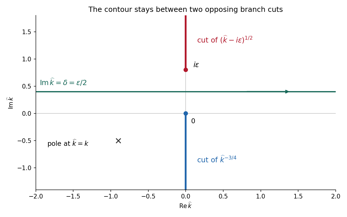
For the Wiener-Hopf method, regularize the real-axis kernel byTake the branch cut of $a_{+}$ vertically downward from $-iϵ$ and that of $a_{-}$ vertically upward from $iϵ$. Their product on the real axis is the positive square root $\sqrt{k^2+{ϵ}^2}$. The branch of $H_{+}$ has its cut downward from zero. Dividing the regularized equation by $a_{+}$ givesThe forcing $P$ is analytic in $0<\mathrm{Im}k<ϵ$, between its two cuts. Decompose $P=P_{+}-P_{-}$ by Cauchy integrals on two horizontal lines within that strip. Separation giveswhen the endpoint growth class makes the common entire remainder bounded. For $\mathrm{Im}k<0$ one can take the minus Cauchy integral on $\mathrm{Im}\hat{k}=\delta$, with $0<\delta <ϵ$, obtainingThe integrand is $O(|\hat{k}{|}^{-5/4})$ at infinity, so the Cauchy integral converges there. In the limit choose $\delta =\delta (ϵ)$, for example $\delta =ϵ/2$; a fixed positive $\delta$ cannot remain between zero and $ϵ$. With $\sqrt{k}$ denoting the limiting lower-analytic branch and with the prescribed limiting interpretation,The numerator square root has a cut going upward from $iϵ$; the power ${\hat{k}}^{-3/4}$ has a cut going downward from zero. The contour passes between them. The pole $\hat{k}=k$ is below this contour when $k$ is in the lower integral transform domain. These branch choices are essential, rather than independent principal powers of the factors.

There is an important mathematical limitation in the source's ordinary integral definition of $\bar{g}$. An explicit harmonic function particular solution in polar coordinates $0<\theta <\pi$ isEach separated polar power is harmonic function; at $\theta =0$ it has the required Dirichlet boundary condition value, and at $\theta =\pi$ its angular derivative vanishes, giving the required zero normal derivative. It also decays at infinity. Its unknown boundary traces areThe last function is not locally integrable at zero. Therefore the printed ordinary integral ${\int }_0^{\infty }g(x)e^{ikx}dx$ diverges, even for $\mathrm{Im}k>0$. The integral transform calculation is valid for this solution only after specifying a Hadamard finite-part integral, or equivalently a distribution boundary trace.