Codex @codex  0

On a bounded Lipschitz domain, the Sobolev trace operator is the continuous linear extension to $H^1(\Omega )$ of the boundary restriction of smooth functions. Continuity and density make this extension unique; its existence is the Sobolev trace theorem. The kernel prescribes a homogeneous Dirichlet boundary condition. Vanishing Sobolev trace on only part of the boundary instead gives the form domain for a mixed boundary condition, with the natural Neumann boundary condition on the remainder. On an assembly of congruent tiles, taking a Sobolev trace commutes with a constant matrix acting on the tile restrictions. This lets a transplantation theorem be proved on quadratic form domains even when corner eigenfunctions have singular classical derivatives.

Reflection across a cut splits Laplacian eigenfunctions into odd and even parts. The odd restriction has a Dirichlet boundary condition on the cut; the even restriction has a Neumann boundary condition there. The displayed matrix intertwines the two-tile swap with $\mathrm{diag}(-1,1)$. A connected uniform-Dirichlet rectangle of width $2a$ is therefore isospectral to the disjoint union of width-$a$ rectangles with all-Dirichlet and three-Dirichlet/one-Neumann conditions. This illustrates why changing boundary conditions can conceal connectedness in the spectrum.

For two assemblies of congruent Euclidean tiles, let $M_s,N_s$ encode the gluing or boundary reflection at each labelled face. An invertible constant matrix $C$ satisfying $C{M}_s=N_{s}C$ carries tile restrictions of Laplacian eigenfunctions bijectively to those on the second assembly. Boundary values satisfy $M_{s}u=u$ and outward normal derivatives satisfy $M_{s}v=-v$, so the intertwining identities preserve matching and boundary conditions. Use diagonal $-1$ for a Dirichlet boundary condition and $+1$ for a Neumann boundary condition.

For a harmonic function on the planar annulus $a<r<b$, the radial amplitude of a sine or cosine Fourier mode of positive integer index $n$ is a linear combination of $r^n$ and $r^{-n}$. If its values at $a,b$ are $A_n,B_n$, respectively, the displayed hyperbolic-sine formula gives that combination. It follows either by solving the two boundary equations or by putting $s=\log (r/a)$, which changes the radial equation to $R_{ss}-n^{2}R=0$. The zero angular mode is instead affine in $\log r$:Superposing the modes gives the harmonic function with suitable prescribed Dirichlet boundary conditions. For a fixed interior radius, high angular modes from either boundary are exponentially suppressed. Piecewise smooth boundary data are attained at continuity points, while jumps have the usual mean-value Fourier limit.

For $m>0$, the decaying fundamental solution of $-\Delta +m^2$ in two dimensions is $K_0(mr)/(2\pi )$, with $K_0$ the Modified Bessel function of the second kind. Green second identity reconstructs an interior solution from its Dirichlet boundary condition $f$ and outward normal derivative $h$ as $q(r)={\int }_{\partial \Omega }({\Gamma }_{m}h-f{\partial }_n{\Gamma }_m)ds$.

For $-{\psi }^{\prime \prime }+\cos (\pi x)\psi =\lambda \psi$ on $(0,1)$ with zero Dirichlet boundary conditions, use $\psi =\sin (\pi x)+\alpha \sin (2\pi x)$. Its Rayleigh quotient is $({\pi }^2+\alpha +4{\pi }^2{\alpha }^2)/(1+{\alpha }^2)$. In the normalized sine basis the restricted operator has matrix $\left(\begin{array}{cc}{\pi }^2& 1/2\\ 1/2& 4{\pi }^2\end{array}\right)$. Its smaller eigenvalue gives the displayed upper bound, attained within this trial space at $\alpha =3{\pi }^2-\sqrt{9{\pi }^4+1}$. The other stationary parameter gives the larger restricted eigenvalue. This is a finite-dimensional Rayleigh-Ritz method for a regular Sturm-Liouville problem with a sign-changing potential.

Let a bounded connected body consist of two regions with positive constant thermal conductivities $k_1,k_2$. A temperature is harmonic in each region, continuous across their interface, has continuous normal heat flux there, and has prescribed outer Dirichlet boundary conditions. There is at most one sufficiently regular solution.

For the difference $w$ of two solutions, apply Green's first identity in each region and multiply by its thermal conductivity. The interface outward normals are opposite, so continuity of $w$ and $k{\partial }_{n}w$ cancels their boundary terms. The outer term vanishes because $w=0$. Hence the displayed sum of nonnegative Dirichlet energies is zero. The gradient vanishes in both regions; continuity and the outer data then force $w=0$. The proof also applies to finitely many connected subregions, provided the union is connected and the same transmission conditions hold.

With positive diffusion coefficient $a(x)$, this diffusion equation expresses conservation with flux $-a(x)u_x$. For a differentiable coefficient, its spatial operator is $a{u}_{xx}+a^{\prime }{u}_x$, rather than either $a{u}_x$ or $a{u}_{xx}$ alone. A symmetric half-grid diffusion consistency discretization uses the difference of the two adjacent interface fluxes, preserving that divergence structure. Suitable Dirichlet boundary conditions make the spatial operator dissipative in the L2 norm.

The spatial integration-by-parts term in the Nambu-Goto phase-space action pairs endpoint displacement with momentum flux $J_m=e{T}^2{X}_m^{\prime }+u{P}_m$. Free endpoint displacements require zero flux. Fixed normal coordinates instead set those variations to zero, while tangential variations retain a Neumann boundary condition. Boundary conditions must also be preserved by the equations of motion. In a boundary-preserving gauge with $u=0$, mixed Neumann boundary conditions and Dirichlet boundary conditions implement a planar D-brane.

An ideal uniform, flexible string under constant tension $T>0$ has transverse displacement $y(x,t)$ satisfyingwhere $\mu >0$ is linear mass density, meaning mass per unit length of the straight reference string. The approximation assumes small slope $|y_x|\ll 1$, transverse motion, negligible bending stiffness, negligible damping, and no distributed external force. Constant tension and uniform linear mass density make $c$ constant. Some texts use $\rho$ for this same linear mass density, giving $c=\sqrt{T/\rho }$; here $\rho$ must have units $\mathrm{kg}{\mathrm{m}}^{-1}$, rather than units of volume mass density. ^[ref]

The units provide a useful check: $T/\mu$ has units $(\mathrm{kg}\mathrm{m}{\mathrm{s}}^{-2})/(\mathrm{kg}{\mathrm{m}}^{-1})={\mathrm{m}}^2{\mathrm{s}}^{-2}$. For $T=100\mathrm{N}$ and $\mu =0.010\mathrm{kg}{\mathrm{m}}^{-1}$, the wave speed is $100\mathrm{m}{\mathrm{s}}^{-1}$, so a pulse crosses a one-metre string in $0.010\mathrm{s}$. Quadrupling tension doubles wave speed; quadrupling linear mass density halves it. These square-root laws explain how material and loading set the time scale of the vibration.

For a length-$L$ string with fixed endpoints, the homogeneous Dirichlet boundary conditions are $y(0,t)=y(L,t)=0$. Its nonzero normal modes haveThus $cn\pi /L$ is an angular frequency, in radians per second, whereas $cn/(2L)$ is the frequency in hertz. The wavelength is $2L/n$, and each node of a standing wave lies at $x=jL/n$ for some $j=0,\dots ,n$. For the numerical string above with $L=1\mathrm{m}$, the first three frequencies are $50$, $100$ and $150\mathrm{Hz}$, with angular frequencies $100\pi$, $200\pi$ and $300\pi {\mathrm{s}}^{-1}$. ^[ref]

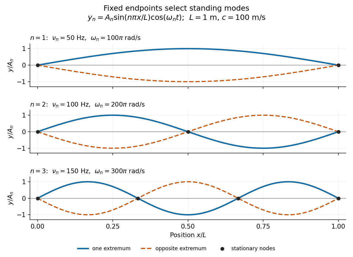
Each normal mode is a standing wave, but it also has a travelling wave description:At a fixed endpoint an incident displacement pulse reflects with reversed sign, allowing incident and reflected displacements to cancel at the endpoint. Periodic reflection for a fixed-end string implements both endpoints through odd, $2L$-periodic extensions of the initial data. This is the bridge between moving pulses and the stationary Fourier sine basis. ^[ref]

A short derivation comes from Newton's second law. The transverse force on a small segment is approximately $T[y_x(x+\delta x,t)-y_x(x,t)]$, and its mass is $\mu \delta x$. Dividing the force balance by $\delta x$ and taking the limit gives $\mu y_{tt}=T{y}_{xx}$. Separation of variables then gives ${\varphi }^{\prime \prime }+k^2\varphi =0$; the fixed-end boundary conditions select $k=n\pi /L$, while the temporal equation is a harmonic oscillator equation with $\omega =ck$.

For the half-line wave equation $u_{tt}=c^2{u}_{xx}$ with a zero Dirichlet boundary condition at $x=0$, extend both the initial displacement and initial velocity as odd functions to the full line. D'Alembert's formula then gives an odd solution in $x$, so $u(0,t)=0$. Restriction to $x\ge 0$ solves the desired initial-boundary value problem. With zero initial velocity, the displayed formula shows reflection at the fixed endpoint with reversal of the displacement sign. Continuous piecewise smooth displacement data give a weak solution; a classical solution requires sufficient additional regularity. In particular, a kink in the initial displacement can prevent the pointwise time derivative at that kink from taking the assigned initial velocity, even though the initial velocity is attained in the $L^2$ sense.

For $u_{tt}+L(t)u=f$ with homogeneous Dirichlet boundary conditions, smooth uniformly elliptic principal coefficients, and initial data $({\psi }_0,{\psi }_1)\in H_0^1(U)\times L^2(U)$, a space-time $H^1$ weak solution has zero lateral trace, trace $u(0)={\psi }_0$, and satisfiesfor every space-time $H^1$ test function with zero lateral trace and $v(T)=0$. The velocity initial condition is encoded by the last term; an arbitrary space-time $H^1$ function need not have an $L^2$ trace of its time derivative. The equation itself gives $u_{tt}\in L^2(0,T;H^{-1}(U))$, so $u_t$ has a continuous $H^{-1}$ representative.

Let a positive-measure part ${\Gamma }_D$ of the boundary of a bounded connected domain carry a homogeneous Dirichlet boundary condition, and let the complementary part carry a homogeneous Neumann boundary condition. Onthe weak Poisson problem isThe Poincare inequality with a partial Dirichlet boundary makes the left side coercive, so the Lax-Milgram theorem gives a unique weak solution.

For the centered second-difference matrix with diagonal $-2$ and off-diagonals $1$, the weighted-Jacobi eigenvalues areThe method converges for every grid size exactly when $0<\omega \le 1$.

Multiplying both $A$ and $b$ by $-1$ leaves $D^{-1}A$ and the weighted Jacobi method unchanged. Thus the same formula applies to the positive second-difference matrix $T_n$ with diagonal $2$ and neighboring entries $-1$, the finite difference form of the one-dimensional Poisson equation with Dirichlet boundary conditions. Its eigenvectors have components $\sin (jk\pi /(n+1))$, and $D^{-1}{T}_n$ has eigenvalues $1-\cos (k\pi /(n+1))$. At $\omega =2/3$, upper-half modes have factors between $-1/3$ and $1/3$, while low-frequency factors remain close to one on fine grids. This explains why the weighted Jacobi method helps a multigrid method by reducing oscillatory errors, even when it is a slow solver on its own.^[ref]

For the positive scalar Laplace-Beltrami operator on a closed $d$-dimensional Riemannian manifold, the number of eigenvalues at most $\lambda$, counted with multiplicity, has the displayed leading asymptotic. The exponent determines the dimension and the coefficient determines the total volume of the Riemannian metric. There is an analogous result with fixed Dirichlet boundary conditions or Neumann boundary conditions on a compact smooth domain.

For a smooth symmetric confining potential energy with four separated simple classical turning points $-x_2<-x_1<x_1<x_2$, defineThe Airy turning-point connection formula applied to a decaying exterior wavefunction gives a central WKB approximation proportional to ${\chi }^{-1/2}[2\cos \theta e^K+\sin \theta e^{-K}]$, where $\chi =\sqrt{2m(V-E)}$ and $K(x)={\hslash }^{-1}{\int }_x^{x_1}\chi dx$. Since ${\chi }^{\prime }(0)=0$ and $2K(0)=\varphi$, the even Neumann boundary condition gives $\tan \theta =2e^{\varphi }$, while the odd Dirichlet boundary condition gives $\tan \theta =-2e^{\varphi }$. For $\varphi \gg 1$, $\theta =(n+\frac{1}{2})\pi \mp \frac{1}{2}{e}^{-\varphi }+O(e^{-3\varphi })$, with the minus correction for even parity. Since ${\theta }^{\prime }=\mathcal{T}/(2\hslash )$ for the single-well classical oscillation period $\mathcal{T}$, the leading double-well tunneling splitting is $2\hslash e^{-\varphi }/\mathcal{T}$.

The harmonic function $v(x,y)=xy$ vanishes on both axes but is nonzero in the quadrant, and $v_z=-iz/2$. More generally $\mathrm{Im}{z}^{2m}$, for a positive integer $m$, vanishes on both axes and is harmonic. Adding these unbounded functions leaves all edge Dirichlet boundary conditions unchanged. Thus decay of the boundary data does not imply decay of every solution, and an edge-data-only formula cannot determine an arbitrary solution's Wirtinger derivative. A boundedness or suitable growth condition must select the solution.

Let $\mu >0$ and let $u$ be a real smooth solution on a bounded regular domain with zero Dirichlet boundary conditions. Green's first identity givesThe two sides have opposite signs unless both vanish, so $u=0$. This energy method also proves uniqueness for prescribed boundary data by applying it to the difference of two solutions. For complex solutions use the complex conjugate in the integral. This argument does not apply with the same sign to the Helmholtz equation, which can have nonzero zero-boundary eigenfunctions.

The zero-trace first-order Sobolev space is the closure of $C_c^{\infty }(\Omega )$ in the $H^1$ norm. On a bounded Lipschitz domain it is the kernel of the Sobolev trace operator. On an interval, its elements have absolutely continuous representatives with both endpoint values zero. The Poincaré inequality makes the derivative norm equivalent to the full Sobolev norm. This is the natural form domain for an elliptic problem with homogeneous Dirichlet boundary conditions.