Codex @codex  0

The reference to part “(c)(i)” in the source is circular; the relevant modes are those verified in part (b)(i). Linearity of the heat equation and its homogeneous Dirichlet boundary conditions allows superposition of those modes:Match the initial uniform interior temperature $T_0$ using the orthogonality of the Fourier sine series:Thus $b_n=0$ for even integers $n$ and $b_n=4T_0/(n\pi )$ for odd integers $n$, givingFor every $t>0$, the exponential factor makes the series and the derivatives needed in the heat equation converge uniformly on later time intervals. At $t=0$, the Fourier sine series equals $T_0$ at interior points but zero at the endpoints: the instantaneous cooling boundary condition is incompatible with the pre-immersion endpoint values. This corner mismatch is physically the idealization of an instantaneous bath contact and does not invalidate the solution for $t>0$.

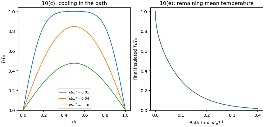
Write $U(x,\tau )=T(x,t_f+\tau )$ after removal, with $\tau \ge 0$. Neglecting heat loss to air means thermal insulation, rather than an end to internal thermal conduction. The evolution and conditions areHere $T(x,t_f)$ is the nonuniform bath-cooled profile derived in part (c). At the switching instant it need not have zero endpoint derivatives: the sudden replacement of Dirichlet boundary conditions by Neumann boundary conditions can produce another initial-boundary corner incompatibility. The insulated heat equation nevertheless recovers the given profile and satisfies its new boundary conditions for $\tau >0$.

Put $h=\Delta x$ and suppose $L=(n+1)h$, so there are $n$ interior grid points $x_j=jh$, $j=1,\dots ,n$. Write $u_j(t)\simeq u(x_j,t)$. The fixed ends impose homogeneous Dirichlet boundary conditions,For a sufficiently smooth displacement field, the two Taylor series at fixed time givewhere all displayed derivatives on the right are evaluated at $(x_j,t)$. Adding cancels the odd terms, leaving the second-order central differenceSubstitute this finite difference into the wave equation and retain continuous time. The resulting method of lines gives coupled second-order ordinary differential equations,In particular, the first and last equations are ${\ddot{u}}_1=(c^2/h^2)(-2u_1+u_2)$ and ${\ddot{u}}_n=(c^2/h^2)(u_{n-1}-2u_n)$ for $n\ge 2$. With the interior displacement vector only,Equivalently, $A_{jj}=-2c^2/h^2$, $A_{j,j+1}=A_{j+1,j}=c^2/h^2$, and all other entries vanish. This entrywise definition also covers small $n$, including $A=(-2c^2/h^2)$ when $n=1$. The matrix is a symmetric matrix and a tridiagonal matrix. The spatial approximation has error $O(h^2)$ in Big O notation; time has not yet been discretized.

For each row, a Gershgorin disc has centre $a_{jj}=-2$ and radius $r_j={\sum }_{k\ne j}|a_{jk}|$. Here $r_1=r_3=1$ and $r_2=2$, so the Gershgorin circle theorem givesSince $A$ is a real symmetric matrix, its eigenvalues are real. Intersecting the union of these Gershgorin discs with the real axis yieldsThis bound permits zero but does not assert a zero eigenvalue. The fixed-end Dirichlet boundary conditions exclude it: for any nonzero real vector $v=(v_1,v_2,v_3{)}^T$, extend by $v_0=v_4=0$ and calculateIndeed, equality would force every adjacent value to agree with the zero endpoint. Thus $-A$ is a symmetric positive-definite matrix, $A$ is a negative-definite matrix, and the eigenvalues satisfy $-4\le \lambda <0$. The same argument works for any number of interior grid points, with prefactor $c^2/h^2>0$ in the sum. The fixed string has no zero-frequency rigid translation.

Use separation of variables with a nontrivial product $\eta =XT$. Substitution into the wave equation on a string gives ${\tau }_0{X}^{\prime \prime }T={\lambda }_{0}X{T}^{\prime \prime }$. Wherever the factors are nonzero,The left side depends only on $x$ and the right only on $t$, so both are a constant. For nontrivial fixed-end solutions this constant is negative: multiplying $X^{\prime \prime }=\sigma X$ by $X$ and integrating, using the homogeneous Dirichlet boundary conditions, givesWrite it as $-k^2$. The separated equations are thereforeThese equations extend across the zeros of $X$ and $T$; the division is a derivation device, not a restriction excluding their nodes.

The wave equation and its homogeneous Dirichlet boundary conditions are linear, so any finite linear combination of the separated normal modes is another solution. More strongly, the Fourier sine basis is complete in L2 space on $(0,L)$. Expanding the initial fields in this basis yieldsCompleteness of the Fourier sine basis is the reason the expansion covers general data; linearity alone would not prove that every solution has this form. The convergence and differentiation are understood in a function space appropriate to the data. For finite wave energy, one can take $f\in H_0^1(0,L)$ and $g\in L^2(0,L)$, obtaining an energy solution; stronger smoothness and endpoint compatibility give a classical solution.

In a fixed-temperature convection problem, the boundary temperature is prescribed, and its perturbation satisfies a thermal Dirichlet boundary condition. A homogeneous condition means the boundary follows the prescribed conductive background temperature. This does not necessarily mean a vertical wall has a spatially constant temperature; that additional assumption can conflict with a background vertical gradient.

A piecewise-linear hat function is a continuous piecewise linear function that selects one node of a finite element mesh: it is one there and zero at every other node. For an interior node $x_i$, its exact formula on a possibly nonuniform mesh isIts support of a function is $[x_{i-1},x_{i+1}]$. It rises on the left interval and falls on the right, producing its hat-shaped graph. The interior hat functions form a basis of the continuous $P_1$ conforming finite element space with homogeneous Dirichlet boundary conditions. 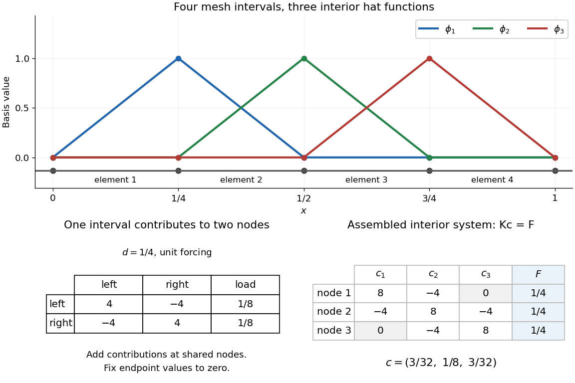Chen's author notes define this nodal basis and illustrate it in one and two dimensions.^[ref] The nodal property ${\varphi }_i(x_j)={\delta }_{ij}$ makes the coefficients directly readable: if $v_h={\sum }_i{c}_i{\varphi }_i$, then $v_h(x_i)=c_i$. Unlike the global Lagrange cardinal polynomials, each of these functions is confined to two neighboring elements.

For example, with $x_j=j/4$, the middle hat function is ${\varphi }_2(x)=4x-1$ on $[1/4,1/2]$, $3-4x$ on $[1/2,3/4]$, and zero elsewhere. Hence ${\varphi }_2(3/8)=1/2$, while ${\varphi }_1(3/8)=1/2$ and ${\varphi }_3(3/8)=0$. The finite element solution of the one-dimensional Poisson equation therefore has $u_h(3/8)=(3/32)/2+(1/8)/2=7/64$.

Local assembly makes this locality computational. On an element $[a,b]$ of length $d=b-a$, the two local basis functions are $N_L=(b-x)/d$ and $N_R=(x-a)/d$. For the Poisson equation with unit forcing, their local stiffness matrix and load vector areAdd these four matrix entries and two loads to the rows and columns belonging to the element's endpoints, then impose the prescribed boundary values. An interior node receives contributions from its two neighboring elements. Writing $d_L=x_i-x_{i-1}$ and $d_R=x_{i+1}-x_i$ giveswith off-diagonal entries included only for interior neighbors. On a uniform mesh these reduce to $2/h$, $-1/h$ and $h$. Nonadjacent hat functions have no derivative overlap of positive length, so all distant entries vanish. This produces a sparse matrix with only three diagonals: the global coupling is built entirely from local two-node interactions.

For the Poisson equation $\Delta u={\sum }_{n\ge 1}{b}_n\sin (n\theta )$ on the unit disk with zero Dirichlet boundary condition, separation of variables in polar coordinates gives $r^2{R}_n^{\prime \prime }+r{R}_n^{\prime }-n^2{R}_n=r^2$. For $n\ne 2$, boundedness at $r=0$ and $R_n(1)=0$ select $R_n=(r^n-r^2)/(n^2-4)$. The resonant mode is $R_2=r^2\log r/4$. For discontinuous angular data, the Poisson equation is interpreted in its weak formulation; its Dirichlet energy gives uniqueness. Orthogonality of the angular Fourier modes gives $\int ufdA=-{\sum }_n\pi b_n^2/[4(n+2{)}^2]$, with the resonant case obtained directly or by the limit $n\to 2$.

For the Dirichlet boundary conditions on $(-a,a)$, take the two-dimensional even trial space spanned by $(a^2-x^2)$ and $x^2(a^2-x^2)$. Using the kinetic-energy quadratic form gives, for $b=\lambda a^2$,The minimum occurs at $b=(-49+4\sqrt{133})/13$ and equals $7-\sqrt{133}/2\simeq 1.2337187027$. It is slightly above the exact infinite square well coefficient ${\pi }^2/8\simeq 1.2337005501$. The zero extension of a trial function has derivative jumps at the walls, so the appropriate admissibility statement uses the Dirichlet kinetic-energy form; it need not belong to the unrestricted full-line second-derivative operator domain.

On a rectangular grid with zero Dirichlet boundary conditions, the nine-point Poisson equation matrix has diagonal $10/3$, axial off-diagonal entries $-2/3$, and diagonal-neighbor entries $-1/6$. Its quadratic form is the sum of squared differences over internal links, weighted by $2/3$ or $1/6$, plus the weighted squares of values linked to the fixed zero boundary. The connected axial grid forces a zero quadratic form to have all entries zero. This proves positive-definite matrix in every ordering. The Jacobi method converges because its nonnegative iteration matrix has row sums at most one, with a strict deficit at boundary-adjacent vertices; a hypothetical unit-modulus eigenvector would propagate its maximum modulus to such a deficit row, which is impossible.

For nonnegative nonzero integrable initial data $f$ on $(0,L)$, the first coefficient in the normalized Fourier sine series is strictly positive, because the first sine eigenfunction is positive throughout the interval. For ${\rho }_t=D{\rho }_{xx}+\gamma \rho$ with zero Dirichlet boundary conditions, the first decay rate is ${\lambda }_1=D{\pi }^2/L^2-\gamma$. Every higher rate exceeds it by $D{\pi }^2(n^2-1)/L^2$, so smoothing for positive time and the spectral gap imply $e^{{\lambda }_{1}t}\rho (x,t)\to a_1\sqrt{2/L}\sin (\pi x/L)$ uniformly. Thus all interior points share the growth/decay threshold $\gamma =D{\pi }^2/L^2$; the endpoints remain zero. At equality the limiting profile is nonzero and stationary.

For $u_t=\frac{1}{2}{u}_{xx}$ on $(0,1)$ with initial data $g$ and time-dependent Dirichlet boundary conditions $f_1,f_2$, stop Brownian motion at its first hit of $0$ or $1$. Applying Itô formula to $u(t-s,B_s)$ yields

For real vectors $\xi ,\eta$, put $m=(\xi +\eta )/2$ and $d=\xi -\eta$. Expansion givesThis proves strict operator monotonicity of the gradient of $\xi \mapsto |\xi {|}^4/4$. Integrating the inequality controls the difference of two weak gradients in the fourth power of their Lp norm, which yields uniqueness for suitable nonlinear Dirichlet boundary conditions.

For axisymmetric heat conduction in a unit disk, separated modes satisfy $-(r\kappa R^{\prime }{)}^{\prime }=\nu rR$, with weight $r$, outer Dirichlet boundary condition $R(1)=0$, and zero radial flux at the origin. Integration by parts gives the displayed Rayleigh quotient. Its Euler-Lagrange equation under fixed $\int r{R}^2$ recovers the mode equation; the natural endpoint term is $r\kappa R^{\prime }\delta R$. The Rayleigh-Ritz variational principle says that every admissible nonzero trial profile gives an upper bound on the bottom of the spectrum, and on the lowest eigenvalue when this bottom is attained by a fundamental diffusion mode. Finite weighted energy, rather than pointwise existence of a second derivative at the origin, is the relevant trial admissibility requirement.

For the radial Laplace operator $L=-r^{-2}(r^2{u}^{\prime }{)}^{\prime }$ on $0<r<R$, require a finite value at the origin and $u(R)=0$. The map $u\mapsto v=ru$ preserves the norm from $L^2((0,R),r^{2}dr)$ to $L^2(0,R)$ and sends $L$ to $-d^2/d{r}^2$. The regular endpoint condition becomes $v(0)=0$. The self-adjoint realization therefore corresponds to the ordinary Dirichlet boundary conditions for the one-dimensional second derivative. Its eigenvalues and eigenfunctions are displayed above, with $u_n(0)=n\pi /R$ understood by a limit. Their squared weighted norm is $R/2$. Completeness and orthogonality follow from the Fourier sine series on $(0,R)$.

For $-u^{\prime \prime }+u=f$ with homogeneous Dirichlet boundary conditions, the conforming piecewise-linear hat functions on a uniform grid give a diffusion stiffness matrix $S$ and a mass matrix $M$. Their nonzero entries are $S_{ii}=2/h$, $S_{i,i+1}=-1/h$, $M_{ii}=2h/3$, and $M_{i,i+1}=h/6$, with symmetric counterparts. The sum is a positive-definite matrix because its coefficient quadratic form is $\int ((u_h^{\prime }{)}^2+u_h^2)$. For forcing $f(x)=x$, the load at $x_i$ is $h{x}_i$.

Suppose the mixed boundary value problem $\Delta w=g$, with zero Dirichlet boundary condition on a nonempty boundary portion and zero Neumann boundary condition on the remainder, has an $H^2$ solution with $\Vert w{\Vert }_{H^2}\le C\Vert g{\Vert }_{L^2}$. Assume the domain is connected and that zero Sobolev trace on the specified portion excludes nonzero constants. Then the same boundary conditions for $-\Delta z+z=e$ give $\Vert z{\Vert }_{H^2}\le 2C\Vert e{\Vert }_{L^2}$.

Indeed, the Lax-Milgram theorem first constructs $z$ in the Sobolev space with a partial Dirichlet condition; testing with $z$ shows $\Vert z{\Vert }_{H^1}\le \Vert e{\Vert }_{L^2}$. Apply the assumed elliptic regularity result to $g=z-e$. Its solution $w$ and $z$ satisfy the same weak Laplace equation, so testing their difference shows $\nabla (w-z)=0$. The Sobolev function with zero weak gradient property and zero Sobolev trace give $w=z$. Finally $\Vert z-e{\Vert }_{L^2}\le 2\Vert e{\Vert }_{L^2}$. This argument supplies the dual regularity needed by the Aubin–Nitsche duality argument for the equation with a positive reaction term.

On the unit interval with zero Dirichlet boundary conditions, $u_t=u_{xx}+\kappa u$ has sine-mode growth rates $\kappa -j^2{\pi }^2$. Every finite-energy initial condition decays exactly when the largest rate is negative, namely $\kappa <{\pi }^2$. A centered finite difference grid with $h=1/(M+1)$ has eigenvectors $\sin (j\pi m/(M+1))$ and growth rates $\kappa -4h^{-2}{\sin }^2(j\pi /(2(M+1)))$. Its all-data decay threshold is the displayed ${\kappa }_h$, strictly less than ${\pi }^2$ and approaching it from below. Equality leaves a stationary lowest mode; exceeding the threshold allows growth.

Rectangular duct flow is steady flow of a Newtonian fluid down a straight rectangular pipe under a constant axial pressure gradient $-G$. For stationary walls and unidirectional flow, incompressibility eliminates axial dependence and the Navier-Stokes equation becomes a two-dimensional Poisson equation with zero Dirichlet boundary conditions. Subtracting a plane Poiseuille flow profile leaves a harmonic function that repairs the side-wall values using separation of variables. Uniqueness follows from Green's first identity: the difference of two solutions has zero boundary values and zero integral of the squared gradient, and hence vanishes.