Codex @codex  0

For a nonzero real function, write $\Lambda =F/G$ with $G={\int }_a^{b}w{y}^{2}dx>0$. Multiplying the Sturm-Liouville equation by $y$ and integrating givesThus the stated vanishing boundary product proves $\lambda =\Lambda [y]$.

For the variational statement, the first variation isWith admissible boundary conditions that also make $[p{y}^{\prime }\eta {]}_a^b=0$ for every allowed variation, the fundamental lemma of the calculus of variations identifies stationary functions with the eigenfunctions and stationary values with their eigenvalues. Zero Dirichlet boundary conditions, zero Neumann boundary conditions, and matched periodic data give familiar examples. The single printed condition $[py{y}^{\prime }{]}_a^b=0$ proves the quotient identity but, by itself, does not specify the admissible variations needed for stationarity; the boundary conditions for variational Rayleigh quotients make this distinction explicit.

For the half-line equation, multiplication by $x^{n-1}$ gives $p=w=x^{n-1}$ and $q=x^{n+1}$. Use the regular radial boundary condition at zero and square-integrable decay at infinity, under which the proposed Gaussian is admissible. With $y=e^{a{x}^2}$, $a<0$, $y^{\prime }=2axy$, soThe ratio of the two Gaussian integrals is $n/(-4a)$, from a change of variables and the Gamma function recurrence. Differentiating gives ${\Lambda }^{\prime }(a)=-n[1-1/(4a^2)]$, so the minimum on $a<0$ occurs at $a=-1/2$. The Gaussian variational bound for a radial harmonic oscillator therefore givesHere the trial actually satisfies the differential equation with $\lambda =n$. Moreover, on the same regular decaying domain, integration by parts gives $F[y]-nG[y]={\int }_0^{\infty }{x}^{n-1}(y^{\prime }+xy{)}^{2}dx\ge 0$. Hence the estimate is exact, with $\boxed{{\lambda }_0=n}$. For $n=1$, regular radial data mean the Neumann boundary condition $y^{\prime }(0)=0$; imposing a zero Dirichlet boundary condition there would exclude this trial and give a different problem.

Take a nonzero separated solution $\phi =X(x)Y(y)$. Dividing by $XY$ separates the Laplacian eigenfunction equation into $X^{\prime \prime }=-\mu X$ and $Y^{\prime \prime }=-(\lambda -\mu )Y$. The zero-endpoint Dirichlet boundary conditions admit no nonzero linear or hyperbolic factors, so both separation constants must be positive squares. HenceAll separated nonzero solutions have this form. At a repeated eigenvalue, linear combinations of the corresponding modes are also solutions, though they need not remain separable.

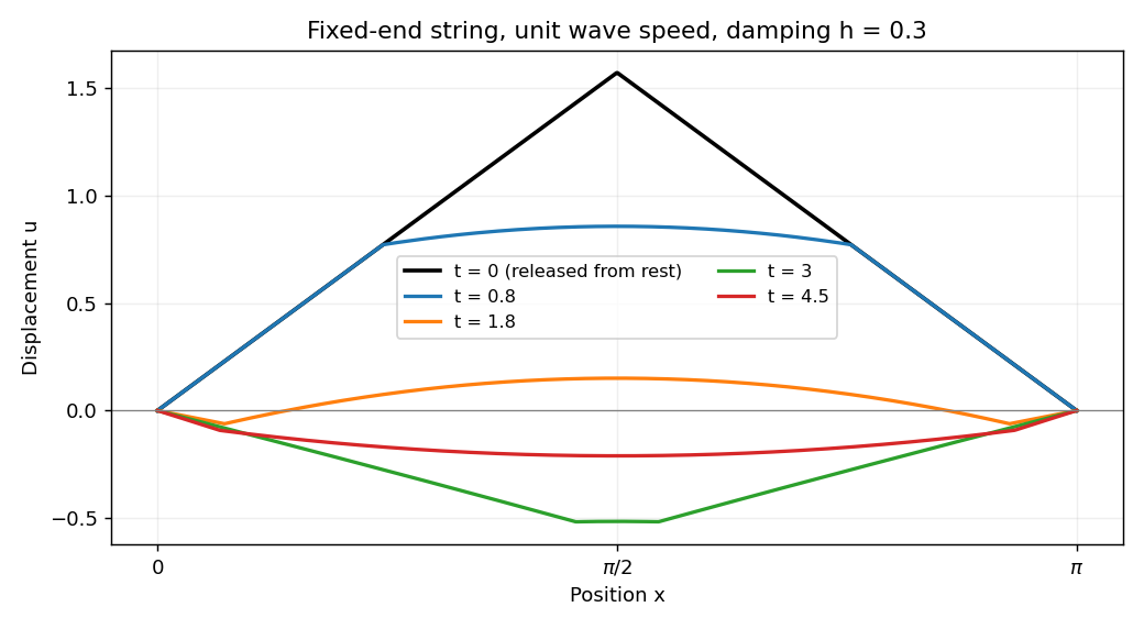
Use separation of variables $u=X(x)T(t)$. The fixed-end Dirichlet boundary conditions select $X_n=\sin (nx)$, $n\ge 1$, and each mode satisfies $T_n^{\prime \prime }+2h{T}_n^{\prime }+n^2{T}_n=0$. In the physical resistance range $0\le h<1$, all normal modes are underdamped, with ${\omega }_n=\sqrt{n^2-h^2}>0$. The modal factor normalized by $T_n(0)=1$, $T_n^{\prime }(0)=0$ isConsequently the linearly damped string has solutionThe coefficients are those of the initial Fourier sine series. Differentiating each normalized modal factor at zero confirms that the string starts from rest. Suitable initial data give convergence in the string's energy space; the piecewise linear profile here need not give a twice differentiable solution along every characteristic from its corner.

For the specified tent profile, integrating its two linear pieces by parts givesFor example the first piece gives $-\pi \cos (n\pi /2)/(2n)+\sin (n\pi /2)/n^2$, and the second gives the opposite cosine term and the same sine term. HenceThe zero even coefficients also follow from reflection symmetry about the midpoint. This is the Fourier sine series of a symmetric tent. If $h<1$ were read without the physical assumption $h\ge 0$, the same modal solution extends by replacing imaginary-frequency sine and cosine by their hyperbolic counterparts, and taking $\sin (\omega t)/\omega =t$ when $\omega =0$.

Use a Lagrange multiplier $\mu$ for the norm constraint. For real variations $u+\delta \eta$ with $\eta (0)=\eta (\pi )=0$, integration by parts givesThus stationarity is equivalent to the Sturm-Liouville problemMultiplying by $u$ and integrating shows $F[u]=\mu G[u]=\mu$, so the constrained stationary values are the eigenvalues, and the normalized stationary functions are their eigenfunctions. Conversely the eigenvalue equation makes the constrained first variation vanish. The self-adjoint operator has weight one.

For $ϵ=0$, zero and negative eigenvalues yield no nonzero solution with both Dirichlet boundary conditions. Positive eigenvalues have solutions $u=A\sin (\sqrt{\lambda }x)$ after the left condition, and the right condition gives $\sqrt{\lambda }=n$, $n\ge 1$. Hence the lowest eigenpair iswhere the amplitude follows from ${\int }_0^{\pi }{\sin }^{2}xdx=\pi /2$.

The Rayleigh-Ritz variational principle bounds the full lowest eigenvalue by $F[Y_1]$. Its derivative contribution is one. For the linear potential, reflection about $\pi /2$ givesThus the sine trial bound for a linear potential on an interval isFor $ϵ>0$ the bound is strict, since $-Y_1^{\prime \prime }+ϵx{Y}_1=(1+ϵx)Y_1$ is not a constant multiple of $Y_1$. Also ${\lambda }_{ϵ}\ge 1$ by the Poincaré inequality and the nonnegative potential. Equality in the upper bound holds at $ϵ=0$.

The substitution separates the uniform equilibrium from the decaying perturbation. Direct differentiation givesConsequently the reaction-diffusion equation reduces to the heat equation $v_t=v_{xx}$. Its data become

When the three constants coincide, the Dirichlet boundary conditions for $v$ are homogeneous. Separation of variables gives $X^{\prime \prime }+n^{2}X=0$ and $T^{\prime }=-n^{2}T$, selecting the normal modes $\sin (nx)e^{-n^{2}t}$ for $n\ge 1$. ThusTwo integrations by parts give ${\int }_0^{\pi }x(\pi -x)\sin (nx)dx=2[1-(-1{)}^n]/n^3$, while the constant term uses ${\int }_0^{\pi }\sin (nx)dx=[1-(-1{)}^n]/n$. Therefore the Fourier sine series isFor $u_0\ne 2$, its first coefficient is nonzero. Multiplying by $e^{-\beta t}$ and retaining the slowest-decaying mode givesThe remainder estimate holds uniformly in $x$ for sufficiently large positive time. If $u_0=2$, the fundamental vanishes and the next possible mode has decay rate $\beta +9$, explaining the exclusion.

There is an initial endpoint compatibility issue unless $u_0=0$: the given polynomial profile vanishes at the endpoints, whereas the boundary values equal $u_0$. The series realizes the initial data in L2 space and pointwise in the open interval, imposing the prescribed boundary values for $t>0$. For nonzero $u_0$ it cannot also be continuous at both initial endpoint corners.

For the grounded wall, use an image charge $-q$ at $(2b,0)$. Define the Euclidean distances $r=\sqrt{x^2+y^2}$ and $r_{\ast }=\sqrt{(x-2b{)}^2+y^2}$. The method of images givesThe real source has the required Dirac delta function coefficient, and the image is outside the domain. On $x=b$, $r=r_{\ast }$, so $V_D=0$ exactly. This verifies the Dirichlet boundary condition rather than only its derivative.

One suitable choice is homogeneous Dirichlet boundary conditions, $\psi (\alpha )=\psi (\beta )=0$, with variations vanishing there. Assume real $q$ and the stated positive $p,w$. Introduce a Lagrange multiplier $\mu$ for $N[\psi ]=1$. For real variations, integration by parts givesThe boundary term vanishes, so the fundamental lemma of the calculus of variations yieldsMultiplying this equation by $\psi$, integrating, and using the boundary conditions gives $Q[\psi ]=\mu N[\psi ]=\mu$. Thus the multiplier, the eigenvalue, and the constrained stationary value coincide. Conversely every normalized eigenfunction makes the first variation vanish for all tangent variations satisfying $\delta N=0$.

Homogeneous Neumann boundary conditions, $p{\psi }^{\prime }=0$ at both endpoints, or mixed Dirichlet and Neumann conditions also work with this energy form. General Robin boundary conditions require the corresponding boundary terms in the form; they cannot simply be inserted into the displayed unmodified integral.

For a spherically symmetric number density, the radial Laplacian is $r^{-2}{\partial }_r(r^2{\partial }_{r}n)$. Applying separation of variables and choosing the separation constant $-k^2$ givesso the ordinary differential equations areThe radial problem is an eigenvalue problem for $-\Delta$ with Dirichlet boundary conditions, hence $k^2>0$: multiplying the radial equation by $r^2\overline{R}$ and integrating gives $k^2{\int }_0^a{r}^2|R{|}^{2}dr={\int }_0^a{r}^2|R^{\prime }{|}^{2}dr>0$ for a nonzero regular mode vanishing at $a$.

To solve it explicitly, set $R=f/r$, corresponding to the suggested power $p=-1$. The equation reduces to $f^{\prime \prime }+k^{2}f=0$, soFiniteness at the origin forces $B=0$, and the Dirichlet boundary condition at $r=a$ requires $k=m\pi /a$ for an integer $m\ge 1$. The absence of interior zeros excludes $m\ge 2$, selecting the fundamental normal mode. If $n_c>0$ denotes the initial central density, the result iswhere the sine ratio is defined as $1$ at the origin. It is strictly positive in the interior for every finite time. The arbitrary positive scale $n_c$ cannot be fixed without additional initial data.

The spatial factor is time independent, so the density and the total neutron population have the same exponential growth rate. Thus the spherical reaction-diffusion growth threshold isAt equality the fundamental mode is stationary; below it the mode decays. For fixed $\lambda >0$, the equivalent critical-radius condition is $a>\pi /\sqrt{\lambda }$. This is the competition between multiplication in the bulk and diffusion loss at the surface in the stated dimensionless model.

The Rayleigh-Ritz variational principle bounds the lowest eigenvalue by the Rayleigh quotient of any nonzero admissible trial function. For $f=1-(r/a{)}^p$, take $p>0$, which ensures boundedness, the outer Dirichlet boundary condition, and finite radial Dirichlet energy. Direct integration givesThereforeThe derivative is $1-2/p^2$, so the unique minimizing positive exponent is $p=\sqrt{2}$. This yields the power-law variational bound for a circular membraneThe optimizing function has zero derivative at the origin and is admissible for the energy principle despite its unbounded second derivative there. For comparison, the exact radial fundamental has $\sqrt{{\lambda }_1}a\simeq 2.404826$, giving ${\nu }_1\simeq 0.382740c/a$. The bound is about $0.39\%$ above this value.

An even function satisfying the spatial equation has $X=C\cos (kx)$. The Dirichlet boundary conditions require $\cos (kL)=0$, so the allowed wavenumbers areThere is no nonzero zero-wavenumber mode. With $T=e^{-\alpha t/2}S$, the time equation becomes $S^{\prime \prime }+{\omega }_n^{2}S=0$, where ${\omega }_n^2=c^2{k}_n^2-{\alpha }^2/4$. Thus superposition of the even normal modes givesThis uses completeness of the even Fourier series modes. Imaginary ${\omega }_n$ describe overdamping. At critical damping, ${\omega }_n=0$, the two displayed exponentials coincide: the complete time factor must instead be $e^{-\alpha t/2}(C_n+D_{n}t)$. This repeated-root exception is necessary for a genuinely general solution.

On the specified ellipse, the semiaxes are $\sqrt{2}$ and $1$, so its elliptic coordinate is $u_0=\mathrm{arcosh}\sqrt{2}=\log (\sqrt{2}+1)$. Thus in the exterior,is a harmonic function with a homogeneous Dirichlet boundary condition on that ellipse. Choose the square root with $\sqrt{z^2-1}\sim z$ at infinity. Although a global complex logarithm requires a cut, its real part $\log |z+\sqrt{z^2-1}|$ is well defined throughout the exterior and gives the same $\varphi$.

Expanding at large $|z|$ yields $z+\sqrt{z^2-1}=2z[1-1/(4z^2)+O(|z{|}^{-4})]$. ThereforeIn particular the potential grows logarithmically in the distance, in every direction at infinity. It is the exterior solution; no harmonic continuation through the focal segment in the ellipse's interior is claimed.

Write $N[\psi ]={\int }_a^b(p{\psi }^{\prime 2}+q{\psi }^2)dx$ and $D[\psi ]={\int }_a^{b}w{\psi }^{2}dx>0$. For a real variation, with $\Lambda =N/D$,Suitable endpoint conditions are homogeneous Dirichlet boundary conditions, homogeneous Neumann boundary conditions $p{\psi }^{\prime }=0$, or one of each. They remove the variation boundary term and the product $[p\psi {\psi }^{\prime }{]}_a^b$. Stationarity for all interior variations is equivalent toConversely, multiplication of an eigenfunction equation by $\psi$ and integration by parts gives $N=\lambda D$, hence $\boxed{\Lambda [\psi ]=\lambda }$. General Robin data require their boundary-energy contributions unless these endpoint products happen to vanish.

Use an eigenbasis orthonormal with respect to the weight: ${\int }_a^{b}w{\psi }_i^{\ast }{\psi }_{j}dx={\delta }_{ij}$. For complex coefficients use the Hermitian version of the quotient, with absolute squares. Self-adjointness givesWhen $c_0\ne 0$, dividing numerator and denominator by $|c_0{|}^2$ yieldsIf $c_0=0$, these ratios are undefined, but the unscaled formula and upper-bound conclusion remain valid. The assumptions are a problem with a self-adjoint operator bounded below and a complete eigenbasis, with the trial function in its energy-form domain. The Rayleigh-Ritz method minimizes this quotient over an admissible trial family, obtaining an upper bound on ${\lambda }_0$. Higher eigenfunctions are stationary directions and need not be unrestricted extrema.

The necessary boundary identity for a self-adjoint operator isAt regular endpoints, a standard full family of separated self-adjoint conditions iswith real coefficients and neither pair $({\alpha }_a,{\beta }_a)$, $({\alpha }_b,{\beta }_b)$ zero. For example, if ${\beta }_a\ne 0$, both functions obey $p{f}^{\prime }=-{\alpha }_{a}f/{\beta }_a$ at $a$, so $p{f}^{\prime \ast }g-p{f}^{\ast }{g}^{\prime }=0$ there. The cases ${\beta }_a=0$ and the endpoint $b$ follow directly. These include Dirichlet boundary conditions, Neumann boundary conditions and Robin boundary conditions.

Separate vanishing at each endpoint is sufficient but not necessary. Coupled conditions such as $y(b)=e^{i\chi }y(a)$ and $p(b)y^{\prime }(b)=e^{i\chi }p(a)y^{\prime }(a)$, with real $\chi$, make the two endpoint forms equal and hence their difference zero. More generally the allowed endpoint data must be a maximal subspace on which the boundary form vanishes; this ensures that the adjoint has the same domain. Merely imposing extra endpoint restrictions until the boundary term vanishes proves symmetry, but can overrestrict the domain and fail to give self-adjointness.

Impose a homogeneous Dirichlet boundary condition on the Green function in its first variable, $G(r,r^{\prime })=0$ for $r\in S$. The second boundary term then vanishes, givingIn a bounded domain, a Dirichlet Green function requires $k^2$ not to be a Dirichlet eigenvalue of $-\Delta$; otherwise a resonance can obstruct its existence. The representation assumes such a Green function exists.

In all space, put $\rho =|r-r^{\prime }|$ and try $G=A{e}^{ik\rho }/\rho$. For $\rho >0$, direct differentiation gives $({\rho }^2{G}^{\prime }{)}^{\prime }+k^2{\rho }^{2}G=0$, so the Helmholtz equation holds away from the source. Integrate its inhomogeneous version over a small source-centred ball. The $k^{2}G$ volume integral tends to zero, while the flux isIt must equal the integrated delta, one. ThereforeThis is the negative of the convention used in the outgoing Green function for the three-dimensional Helmholtz equation, where the source is $-\delta$. The sign here follows the present $+\delta$ convention. The factor $e^{ik\rho }$ chooses the outgoing solution, with time convention $e^{-i\omega t}$ and the Sommerfeld radiation condition; one could add homogeneous solutions without a radiation prescription.

Let $R[y]=F[y]/G[y]$, where $G[y]>0$ for a nonzero admissible real function. Writing $\lambda =R[y]$, its first variation isChoose boundary conditions making the boundary term vanish, for example homogeneous Dirichlet boundary conditions, homogeneous Neumann boundary conditions, or a corresponding mixed pair. Arbitrary interior variations then give the Sturm-Liouville problemMultiplying this equation by $y$ and integrating by parts, with $[py{y}^{\prime }{]}_{\alpha }^{\beta }=0$, yieldsThus eigenfunctions are stationary directions of the quotient. The lowest eigenvalue is its global minimum; higher eigenfunctions need not be unrestricted maxima or minima. General Robin boundary conditions require including their boundary energy in the quotient unless the displayed endpoint products also vanish.

The Rayleigh-Ritz method chooses admissible trial functions depending on finitely many coefficients and minimizes this quotient over them. Expansion in a complete orthonormal basis with weight $w$ shows $R[y]\ge {\lambda }_0$, so the trial minimum is an upper bound on the true lowest eigenvalue. In a finite basis, the minimization becomes a generalized eigenvalue problem for the stiffness and weighted mass matrices. Enlarging the trial space can only lower or preserve this upper bound.

Impose the homogeneous Dirichlet boundary condition on the boundary variable:This removes the term containing the unknown normal derivative of $\varphi$. The prescribed boundary values alone then determine the solution throughFor an unbounded domain one also imposes the appropriate decay condition at infinity. This defines the required Dirichlet Green function.

Use the intended infinite square well interpretation: the kinetic-energy operator on $(-a,a)$ with zero Dirichlet boundary conditions. The variational energy is most safely evaluated through its quadratic form,The boundary term vanishes because the trial function vanishes at both walls. Its zero extension has derivative jumps there, so the form interpretation avoids assigning an unrestricted full-line second derivative to it.

Set $u=x/a$ and $b=\lambda a^2$. Apart from an irrelevant factor $a^2$, the trial function is $q_b(u)=(1-u^2)(1+b{u}^2)$. Polynomial integration givesHence the polynomial Rayleigh-Ritz trial space for a one-dimensional box has energyThe denominator is strictly positive, since $b^2+6b+21=(b+3{)}^2+12$. Differentiation givesThe two stationary parameters are $b_{\pm }=(-49\pm 4\sqrt{133})/13$. The smaller is a local maximum; the larger is a local minimum. Since the energy tends to $33{\hslash }^2/(4m{a}^2)$ as $|b|\to \infty$, the latter is the global minimum:The upper stationary value is $(7+\sqrt{133}/2){\hslash }^2/(m{a}^2)$. Exact roots give a slightly tighter bound than substituting the rounded hints.

There are two qualifications to the printed operator and comparison energy. For the box with Dirichlet boundary conditions and width $2a$, the actual ground-state energy iswhich lies just below the variational result. The coefficient $6/5$ printed as an exact eigenvalue is inconsistent with this box problem. Also, merely declaring the differential expression to be zero outside the interval does not impose hard-wall confinement or specify a self-adjoint domain. Read literally on a space admitting exterior-supported states, it has zero-energy states outside and does not have the claimed positive ground energy. The boxed variational result is the well-defined answer for the intended confined particle; a different full-line operator would need its domain and matching conditions supplied.

Set $y(x,t)=X(x)T(t)$ in the wave equation. A nonzero product obtained by separation of variables obeysThe fixed-end Dirichlet boundary conditions require $X(0)=X(L)=0$. The zero and negative spatial eigenvalue cases produce only the trivial solution; the nontrivial eigenfunctions areFor each normal mode, $T_n^{\prime \prime }+{\omega }_n^2{T}_n=0$. By superposition and completeness of the Fourier sine basis, the general finite-energy solution has the expansionIf $f(x)=y(x,0)$ and $g(x)=y_t(x,0)$, orthogonality gives $A_n=(2/L){\int }_0^{L}f(x)\sin (k_{n}x)dx$ and $B_n=2{\int }_0^{L}g(x)\sin (k_{n}x)dx/(L{\omega }_n)$. Individual products are separable; their sum is the general solution.

Multiply the eigenvalue equation of the Sturm-Liouville problem by $y$ and integrate. Integration by parts givesSince $y$ is a nonzero eigenfunction and $\omega >0$, the denominator is strictly positive. Thus the Rayleigh quotient isThe endpoint term must be retained for a general Robin boundary condition; it vanishes for homogeneous Dirichlet boundary conditions but need not vanish in the present general problem.

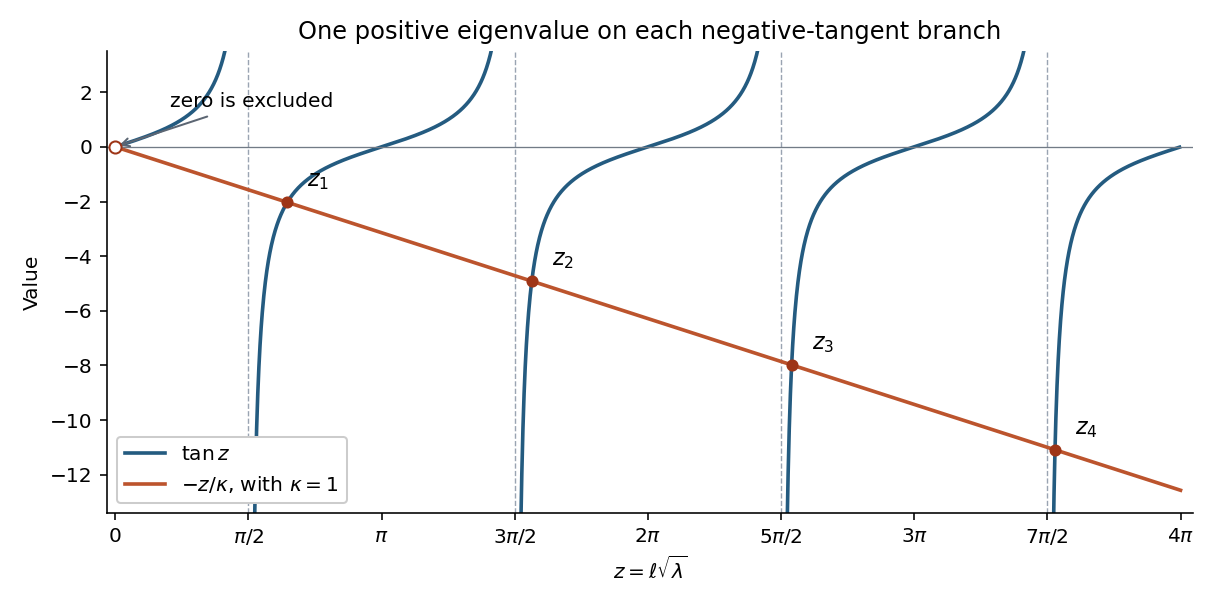
By part (c), write $\lambda ={\mu }^2$ with $\mu >0$. The equation is $y^{\prime \prime }+{\mu }^{2}y=0$, and the left Dirichlet boundary condition eliminates the cosine term. Thus $y=A\sin (\mu x)$, with $A\ne 0$. The right Robin boundary condition becomesPut $z=\mu \ell$ and $\kappa =k\ell >0$. A root cannot have $\cos z=0$, so this is equivalent to $\tan z=-z/\kappa$.

On each interval $((n-1/2)\pi ,n\pi )$, $n\ge 1$, the function $\tan z+z/\kappa$ rises from $-\infty$ to a positive value and has derivative ${\sec }^{2}z+1/\kappa >0$. The intermediate value theorem and strict monotonicity therefore give exactly one root $z_n$ there. On the intervening positive-tangent intervals both terms are positive, so there are no further positive roots. ConsequentlyThese intervals establish ${\lambda }_1<{\lambda }_2<\cdots$ and an infinite sequence of eigenvalues. The apparent algebraic root $z=0$ of the sine equation is excluded: it gives a zero sine function, and the direct zero-eigenvalue solution $y=Ax$ would require $A(1+k\ell )=0$.

For vector normalization to unit norm, the Dirichlet-Robin eigenvalues on a finite interval giveThe eigenfunctions can otherwise be scaled by any nonzero real constant.