Codex @codex  0

Take the spatial interval $0<x<L$ with $L>0$, and write $v=|c|>0$. A separated nonzero solution satisfiesThe zero-endpoint Dirichlet boundary conditions rule out nonzero solutions for $\lambda \le 0$: linear or hyperbolic spatial factors cannot vanish at both ends. For $\lambda >0$, they give $X_n=\sin (n\pi x/L)$ and ${\lambda }_n=(n\pi /L{)}^2$, $n\ge 1$. The temporal factors solve $T_n^{\prime \prime }+{\omega }_n^2{T}_n=0$, with the fixed-end standing wave frequencies ${\omega }_n=n\pi v/L$. Superposition givesThe constants are arbitrary subject to the convergence and regularity required of the solution. For initial displacement $f$ and initial velocity $g$, their Fourier sine series give $A_n=(2/L){\int }_0^{L}f(x)\sin (n\pi x/L)dx$ and $B_n=(2/(L{\omega }_n)){\int }_0^{L}g(x)\sin (n\pi x/L)dx$. Smooth compatible data give classical solutions; weaker data have the corresponding energy interpretation. A negative printed $L$ describes the interval with endpoints reversed and gives the same modes after using its positive length.

For a nonzero separated solution $u=X(x)T(t)$ of the reaction-diffusion equation, substitution and division by $XT$ givesThe two sides depend on different variables, so both equal a separation constant. The homogeneous Dirichlet boundary conditions select a negative spatial constant, written $-k^2$:For $k>0$, $X=A\sin kx+B\cos kx$. The boundary value at zero makes $B=0$; the boundary value at $L$ then requires $kL=n\pi$, with $n=1,2,\dots$. A zero spatial constant gives only a linear function vanishing at both endpoints, hence the zero function; a positive spatial constant similarly gives no nonzero admissible hyperbolic solution. ThereforeBy superposition, the general solution with the stated boundary conditions isThe coefficients are fixed only if initial data are supplied: for $u(x,0)=f(x)$, they are the Fourier sine series coefficients $c_n=(2/L){\int }_0^{L}f(x)\sin (n\pi x/L)dx$. Here they remain arbitrary subject to convergence. Every mode has the ordinary diffusive decay rate plus the additional reaction decay rate one.

With homogeneous Dirichlet boundary condition, the eigenfunctions are $\sin (n\pi x/L)$ and all modes decay. WriteReflection about the midpoint makes every even-$n$ coefficient zero. For odd $n$, putting $u=\pi x/L$ and using the product-to-sum identity givesIn particular $b_1=8T_0/(3\pi )$ and $b_3=-8T_0/(15\pi )$. ThusThis uses the Fourier sine series of a squared sine. The coefficients are $O(n^{-3})$, so the initial series converges uniformly; for $t>0$ the exponential factors also justify termwise differentiation to check the heat equation. Every mode vanishes at both endpoints, and the initial series gives the specified profile. Unlike part (a), there is no constant mode: the temperature tends to zero, with leading long-time term

For a separated nonzero solution $T=f(x)g(y)$, substitution and division by $fg$ givesThe homogeneous Dirichlet boundary conditions impose $g(0)=g(1)=0$. For a nonzero spatial factor, integration by parts gives ${\lambda }^2{\int }_0^1{g}^{2}dy={\int }_0^1(g^{\prime }{)}^{2}dy$, so the separation value is nonnegative. The zero value gives only a trivial linear $g$ under these boundary conditions. The nontrivial separated factors, for $a\ne 0$, are thereforeFor the intended forward diffusion equation, assume $a>0$. The superposition principle gives a Fourier sine series, whose coefficients must expand the initial ramp in the interior:Consequently the standard heat-flow solution isIt satisfies both lateral boundary conditions for $x>0$, and tends to $y$ as $x\downarrow 0$ for $0<y<1$, also converging to the ramp in the L2 norm. The exponential coefficient decay justifies differentiating the series for positive $x$.

There is a genuine incompatibility in the printed data: at $(0,1)$ the lateral condition demands zero while the initial condition demands one. Thus no function satisfies every stated value at that corner. The displayed series solves the usual consistent interpretation with initial data on $0<y<1$ and lateral data for $x>0$; it cannot be continuous at the upper initial corner. This discrepancy is present in the original PDF.

The sign of $a$ is also unstated. If $a=0$, the spatial equation with two zero endpoints forces $T=0$, incompatible with the ramp. If $a<0$, the separated Fourier coefficients grow like $e^{n^2{\pi }^{2}x/|a|}/n$ and fail to be square summable for every $x>0$; these data therefore have no forward solution in the standard L2 space class. The positive-$a$ assumption is essential to the stated heat-flow interpretation.

Boundary form. For real functions and $\mathcal{L}y=-(p{y}^{\prime }{)}^{\prime }+qy$, integration by parts givesThe integral terms containing $p{y}_1^{\prime }{y}_2^{\prime }$ cancel, as do the $q$ terms. This is the Lagrange identity for a Sturm-Liouville operator. The boundary conditions must make this boundary form zero for every admissible pair. Several suitable choices are homogeneous Dirichlet boundary conditions at both endpoints; homogeneous Neumann boundary conditions at both endpoints; one of each; or separated homogeneous Robin boundary conditionswhere each fixed real pair $(\alpha ,\beta )$ is nonzero. At each endpoint the two boundary data vectors are then proportional, making their antisymmetric product zero. Another choice is periodic data $y(a)=y(b)$ and $p(a)y^{\prime }(a)=p(b)y^{\prime }(b)$, which cancel the two endpoint contributions. These domains give the required self-adjoint differential operator in the regular setting.

Eigenfunctions. Set $x=\cos \theta$, $0\le \theta \le \pi$, and $Y(\theta )=y(\cos \theta )$. The chain rule givesThe Chebyshev differential equation therefore becomes $Y^{\prime \prime }+n^{2}Y=0$, with $Y(0)=Y(\pi )=0$. For a positive integer $n$, the first condition excludes the cosine term and the second is satisfied by $\sin (n\theta )$. ThusThere is no nonzero $n=0$ eigenfunction: the transformed solution is linear in $\theta$ and vanishes at both endpoints only if identically zero. Negative $n$ merely repeats a positive mode with the opposite sign, so it is excluded from the indexing of an independent eigenbasis.

Weight and normalization. Multiplying the differential equation by $-1/\sqrt{1-x^2}$ puts it into Sturm-Liouville form:Hence $p=\sqrt{1-x^2}$, $q=0$ and $w=(1-x^2{)}^{-1/2}$. Under $x=\cos \theta$, the measure $w(x)dx$ becomes $-d\theta$, soThereforeThese endpoints are singular because $p$ vanishes and $w$ diverges there, but the weight is integrable. Moreover $p{y}_n^{\prime }=-N_{n}n\cos (n\theta )$ remains finite, so the vanishing values of $y_n$ make the boundary form zero. These are the Dirichlet eigenfunctions of the Chebyshev differential operator, not the first-kind Chebyshev polynomials $\cos (n\arccos x)$, which have nonzero endpoint values.

Variational formulation. Take real $p,q,w$ with $p,w>0$ in the interval, and impose homogeneous Dirichlet boundary conditions, or other suitable conditions that cancel the boundary terms. The functionalhas Euler-Lagrange equationwhich is equivalent to $-(p{y}^{\prime }{)}^{\prime }+qy-\lambda wy=0$. The same construction is constrained stationarity of the energy $\int [p(y^{\prime }{)}^2+q{y}^2]$ subject to $\int w{y}^2=1$, with $\lambda$ a Lagrange multiplier. For fixed zero endpoint values, the variation vanishes at both ends; homogeneous zero-flux conditions also cancel the boundary term $[2p{y}^{\prime }\delta y{]}_a^b$.

Multiplying the differential equation by $y$ and using integration by parts gives the Rayleigh quotientFor a nonzero admissible trial function, $R[y]\ge {\lambda }_0$ by the Rayleigh-Ritz variational principle. The Rayleigh-Ritz method chooses trial functions satisfying the endpoint conditions, often with adjustable coefficients, and minimizes this quotient over that trial family. Expanding $y=\sum c_n{y}_n$ in a normalized eigenbasis shows why the lower bound holds: $R[y]=\sum {\lambda }_n{c}_n^2/\sum c_n^2$, a weighted average of eigenvalues no smaller than the least one.

Radial quadratic trial. The radial problem becomeswhere the printed endpoint notation $y$ refers to $\psi$. Thus $p=w=r^2$ and $q=0$. At the origin the vanishing $r^2$ and regularity of $\psi$ make the boundary term vanish; the weight must be retained in both numerator and denominator.

For a quadratic $\psi =A+Br+C{r}^2$, the derivative condition sets $B=0$ and the outer condition gives $C=-A$. Overall amplitude cancels in the Rayleigh quotient, so take $\tilde{\psi }=1-r^2$. ThenwhileConsequently

Why the estimate is higher. For a regular radial function put $u=r\psi$. Then $u(0)=u(1)=0$, and direct differentiation transforms the equation to $u^{\prime \prime }+\lambda u=0$. Its first mode is $u=\sin (\pi r)$, corresponding to $\psi =\sin (\pi r)/r$ with its continuous value at the origin. Thus ${\lambda }_0={\pi }^2$. The quadratic trial is not proportional to that Spherical Bessel function, so it has nonzero components in higher modes. Its Rayleigh quotient is therefore strictly larger than ${\pi }^2$, in agreement with $21/2>{\pi }^2$.

For the nonconstant boundary data, use separation of variables in polar coordinates and put $\varphi =R(r)\cos 2\theta$. Laplace's equation reduces toThis Cauchy-Euler equation has independent solutions $r^2$ and $r^{-2}$. Unlike a disk containing the origin, the annulus permits both. The zero inner boundary value requires $R=A(r^2-a^4{r}^{-2})$, and the outer value requires $A=V{b}^2/(b^4-a^4)$. HenceSubstituting $r=a$ gives zero, while $r=b$ gives $V\cos 2\theta$. This is the Dirichlet problem on an annulus for one Fourier mode; no other angular mode is needed.

For the changed inner boundary value, use superposition to add a radial harmonic function that is $-V$ at $a$ and zero at $b$. The radial zero-mode equation is $(r{R}^{\prime }{)}^{\prime }=0$, giving $R=C+D\log r$. Imposing the two constant boundary values givesTherefore the second answer isThe logarithmic term is independent of $\theta$, so it changes only the angular average of the electric potential. Both answers are unique for these Dirichlet boundary conditions, by uniqueness for Laplace's equation.

Green identity. With $n$ the outward unit normal, the product rule gives $\nabla \cdot (u\nabla v)=u{\nabla }^{2}v+\nabla u\cdot \nabla v$. Integrating over $V$ and applying the divergence theorem yields Green's first identity:

Uniqueness for nonzero mass. Suppose two real solutions have the same prescribed boundary data, and let $w$ be their difference. The spatial equation called the Klein-Gordon equation in the question is the modified Helmholtz equation, so ${\nabla }^{2}w=m^{2}w$. With $u=v=w$, Green's first identity becomesFor identical Dirichlet boundary conditions, $w=0$ on $S$; for identical Neumann boundary conditions, ${\partial }_{n}w=0$ there. Either makes the right-hand side zero. When $m$ is real and nonzero, both integrands on the left are nonnegative, forcing $w=0$. ThusThis is the required uniqueness assertion; existence is understood for admissible smooth data on a suitable bounded region. Complex-valued solutions obey the same result by treating their real and imaginary parts separately.

Zero mass. For $m=0$, the argument gives $\nabla w=0$, hence $w=C$ on the connected region. Dirichlet boundary conditions still force $C=0$, but Neumann boundary conditions leave an arbitrary additive constant:The prescribed normal data in the zero-mass case must also satisfy ${\int }_S{\partial }_n\Phi dS=0$, by the divergence theorem. For nonzero $m$, that flux can instead equal $m^2{\int }_V\Phi dV$.

Energy minimization. Let $\eta =w-v$ for the two functions in the last part. They share their boundary values, so $\eta =0$ on $S$. Since $v$ is a harmonic function, Green's first identity givesExpand the square in the Dirichlet energy of $w=v+\eta$:The cross term vanishes, soEquality requires $w-v$ to be constant, and the shared boundary values then make it zero. This is the Dirichlet principle: among functions with fixed boundary values, the harmonic function minimizes Dirichlet energy.

Steady state. In the heat equation, time independence makes the second spatial derivative zero. The two endpoint temperatures therefore determine the linear profileInsulation is along the sides; the endpoint reservoirs can still exchange heat with the rod.

Transient solution. Subtract the steady profile before applying separation of variables: let $U=T-T_{0}x/l$. Then $U_t=\nu U_{xx}$, $U(0,t)=U(l,t)=0$ and $U(x,0)=-T_{0}x/l$ for $0<x<l$. Writing $U=X(x)\Theta (t)$ givesThe homogeneous Dirichlet boundary conditions exclude $\mu \le 0$ and select the eigenfunctions $\sin (n\pi x/l)$ with eigenvalues ${\mu }_n=(n\pi /l{)}^2$, $n\ge 1$. Their orthogonality gives the Fourier sine series coefficientsHere integration by parts uses ${\int }_0^{l}x\sin (n\pi x/l)dx=-l^2(-1{)}^n/(n\pi )$. ThusEvery summand satisfies the heat equation and the homogeneous endpoint conditions, while the steady profile supplies the prescribed endpoint values. The initial Fourier sine series equals $-T_{0}x/l$ in the open interval. At $(l,0)$ the initially cold rod and the suddenly imposed hot endpoint are incompatible; the formula describes the prescribed data for $t>0$ and the initial limit at interior points.

Heat absorption. Integrating in $x$ kills the even modes. With $a=\nu {\pi }^2/l^2$, the total heat relative to the initial state isConsequently the net rate of heat absorption isFor each $t\ge \epsilon >0$, any fixed number of differentiated modes is bounded by a polynomial in $n$ times $e^{-a\epsilon n^2}$. These bounds have finite sums, proving absolute convergence, uniform convergence on such time intervals and the validity of the integration and differentiation. In particular the displayed rate is finite for every $t>0$, positive when $T_0>0$, and tends to zero as equilibrium is approached. The same answer follows from the heat equation balance $H^{\prime }=\gamma \nu [T_x(l,t)-T_x(0,t)]$; this subtracts loss at the cold endpoint from input at the hot endpoint.

Multiply the differential equation by $-p(x)$ and compare the coefficients of $y^{\prime \prime }$ and $y^{\prime }$ with $-(p{y}^{\prime }{)}^{\prime }=-p{y}^{\prime \prime }-p^{\prime }{y}^{\prime }$. The required integrating factor satisfies $p^{\prime }=-bp$. Thus one may takeThen $-(p{y}^{\prime }{)}^{\prime }+qy=\lambda wy$, the desired Sturm-Liouville form, with the same homogeneous Dirichlet boundary conditions. A common positive constant multiplying $p,q,w$ is immaterial. For the usual regular Sturm-Liouville problem one also assumes real sufficiently regular coefficients and $d>0$, ensuring $p,w>0$.

For the real Sturm-Liouville operator $\mathcal{L}y=-(p{y}^{\prime }{)}^{\prime }+qy$, two integrations by parts give the Lagrange identity for a Sturm-Liouville operator:Set $u=y_n,v=\tilde{y}$. Both vanish at the endpoints, so the boundary term is zero. Since $\mathcal{L}{y}_n={\lambda }_{n}w{y}_n$,ConsequentlyThis is self-adjointness with the homogeneous Dirichlet boundary conditions, and expresses the Fredholm solvability condition at the eigenvalue ${\lambda }_n$. In this unweighted integral $F_n$ already contains its factor of $w$; adding another weight would be incorrect.

Choose homogeneous Dirichlet boundary conditions, $y(a)=y(b)=0$, and nonzero admissible functions with finite $F$ and positive $G$. Variations obey the same zero endpoint values. At a stationary Rayleigh quotient, set $\lambda =F[y]/G[y]$. ThenThe boundary term vanishes, and the fundamental lemma of the calculus of variations gives the Sturm-Liouville equation $-(p{y}^{\prime }{)}^{\prime }+qy=\lambda wy$. Thus stationary functions are eigenfunctions. Conversely, multiply that equation by $y$ and integrate by parts to obtain $F=\lambda G$; its first variation then vanishes by the same calculation. This proves that stationary values are the corresponding eigenvalues. Homogeneous Neumann boundary conditions also make the displayed boundary terms vanish; general Robin boundary conditions can require a boundary contribution to the quadratic form.

For $p=1$, $q=0$, $w=x$ on $(0,\pi )$, the polynomial trial function $y=x(\pi -x)$ satisfies the endpoint conditions. Its Rayleigh quotient usesso the polynomial estimate is $\boxed{{\lambda }_{\mathrm{poly}}=20/{\pi }^3\simeq 0.64503}$. The trigonometric trial function $y=\sin x$ givesand hence $\boxed{{\lambda }_{\mathrm{trig}}=2/\pi \simeq 0.63662}$. Both are upper bounds on the lowest eigenvalue, by the Rayleigh-Ritz method; neither trial is an exact eigenfunction, so the inequalities are strict.

Their closeness has a useful explanation beyond their similar single-arch shapes. Both trial functions are symmetric under $x\mapsto \pi -x$, forcing ${\int }_0^{\pi }x{y}^{2}dx=(\pi /2){\int }_0^{\pi }{y}^{2}dx$. The reflection-symmetric trials for a linearly weighted Rayleigh quotient therefore reduce this problem to a constant multiple of the ordinary Dirichlet energy quotient. The sine is the best trial within this symmetric class, and the polynomial's value is only a factor $10/{\pi }^2\simeq 1.0132$ larger. The unrestricted lowest eigenfunction can be asymmetric because the weight $x$ is asymmetric.

Choose the stationary solution $w^{\prime \prime }=0$ satisfying $w(0)=0$ and $k{w}^{\prime }(L)=H$. Hence $\boxed{w(x)=Hx/k}$. Subtracting it gives the homogeneous problemThis boundary lifting leaves a Dirichlet boundary condition at one end and a Neumann boundary condition at the other, as in the fixed-temperature and fixed-flux heat equation on an interval.

Multiplication by $x^2$ puts the eigenvalue problem into Sturm-Liouville form, $-(x^2{y}^{\prime }{)}^{\prime }=\lambda x^{2}y$, with weight $x^2$. If $u,v$ correspond to distinct eigenvalues $\lambda ,\mu$, subtract their multiplied equations and integrate to getThe upper boundary term vanishes by the Dirichlet boundary condition. For a bounded solution near zero, $x^2{y}^{\prime }$ has a limit because $(x^2{y}^{\prime }{)}^{\prime }=-\lambda x^{2}y$ is integrable. A nonzero limit would force a $1/x$ divergence in $y$, so that limit is zero; integration then gives $y^{\prime }=O(x)$. The lower boundary term therefore also vanishes, proving the weighted orthogonality.

Set $z=xy$. For $x>0$, $y^{\prime \prime }+2y^{\prime }/x=z^{\prime \prime }/x$, and finiteness of $y(0)$ gives $z(0)=0$. Thus $z^{\prime \prime }+\lambda z=0$ with zero values at zero and $\pi$. The radial Dirichlet spectrum in three dimensions givesThe zero and negative eigenvalues yield only the zero solution under these boundary conditions. Also ${\int }_0^{\pi }{x}^2{y}_n^{2}dx=\pi /2$.

For the forced equation, the same substitution gives $z^{\prime \prime }-\beta z=x$. The Fourier sine series of $x$ on $(0,\pi )$ has coefficientsExpanding $z=\sum c_n\sin nx$ gives $-(n^2+\beta )c_n=b_n$, henceThe value at zero is defined by a limit. In fact $|\sin nx/x|\le n$, so uniform convergence holds even there, by comparison with $2\sum (n^2+\beta {)}^{-1}$. An independent check comes from solving the constant-coefficient equation directly:It satisfies both endpoint conditions and the forcing for $x>0$, and its finite origin limit agrees with the series. For $\beta >0$ the homogeneous boundary value problem has no nonzero solution, so the solution is unique.

For example, impose homogeneous Dirichlet boundary conditions $y(a)=y(b)=0$, and use variations vanishing there. Homogeneous Neumann boundary conditions $p{y}^{\prime }=0$ are another choice removing the boundary terms. Put $N[y]={\int }_a^b(p{y}^{\prime 2}+q{y}^2)dx$, $D[y]={\int }_a^{b}w{y}^{2}dx>0$, and $I=N/D$. At a stationary function let $\lambda =I[y]$. The quotient rule gives $\delta I=(\delta N-\lambda \delta D)/D$. After integration by parts, stationarity under every allowed variation givesso the fundamental lemma of the calculus of variations yields the stated Sturm-Liouville problem. Conversely an eigenfunction with those boundary conditions has $N=\lambda D$ and makes the quotient stationary. The lowest eigenvalue minimizes the Rayleigh quotient under the usual self-adjoint, lower-bounded hypotheses; higher eigenvalues are stationary values with orthogonality constraints when minimizing successively.

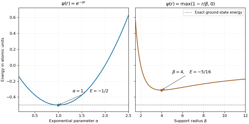
The hydrogen equation becomes $-(r^2{\psi }^{\prime }{)}^{\prime }-2r\psi =2E{r}^2\psi$. Its radial energy quotient is thereforeRegularity at zero and decay at infinity remove the boundary term $r^2\psi {\psi }^{\prime }$. The condition $\psi (0)=1$ fixes an arbitrary amplitude for these trial functions; it is not their three-dimensional probability normalization, which cancels from the quotient.

For $\psi =e^{-\alpha r}$, elementary exponential integrals give $\int r^2{\psi }^{2}dr=1/(4{\alpha }^3)$, $\int r^2{\psi }^{\prime 2}dr=1/(4\alpha )$, and $\int r{\psi }^{2}dr=1/(4{\alpha }^2)$. HenceFor the compactly supported linear trial for hydrogen, the norm, gradient and Coulomb integrals are ${\beta }^3/30$, $\beta /3$, and ${\beta }^2/12$, respectively. ThusThe derivative changes from negative to positive at four, so this is the minimum over positive $\beta$. The quantum variational principle gives upper bounds on the ground-state energy; the exponential trial is better, and in fact $e^{-r}$ satisfies the exact differential equation at $E=-1/2$. It is the nodeless hydrogen ground state in the given units. The linear trial is admissible for the energy quadratic form despite its derivative jump at $r=\beta$; it need not possess a classical second derivative at that point.

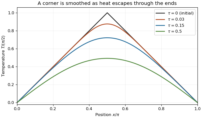
The cooled endpoints impose Dirichlet boundary conditions $\theta (0,t)=\theta (L,t)=0$. The spatial modes are $\sin (n\pi x/L)$. Integrating the initial profile on its two straight segments givesThe heat flow from a triangular initial temperature with height $L/2$ is thereforeEvery nonzero mode decays, so ${\theta }_D\to 0$ as $t\to \infty$. There is no nonzero constant mode compatible with these endpoint temperatures.

For a separated harmonic function $R(r)\Theta (\theta )$ in polar coordinates, single-valuedness forces integer angular frequencies. The radial factors for frequency $m\ge 1$ are $r^m,r^{-m}$, while frequency zero has a constant and $\ln r$. Finiteness at the origin excludes $r^{-m}$ and $\ln r$.

The source's angular factor is $\cos \theta$ in every term, as printed, rather than $\cos (n\theta )$. The power-law angular mode for the planar Poisson equation givesHence, assuming the series permits termwise differentiation, the general finite, single-valued solution isThe arbitrary harmonic series must itself converge to a finite function on the prescribed disk. If ${\alpha }_0\ne 0$, the source has a direction-dependent limit at the origin; the displayed potential still extends finitely there, but the equation at that point is understood weakly rather than as a smooth classical source.

For the special source, a particular potential is $r^3\cos \theta /8$. Its boundary cosine term is canceled by $-a^{2}r\cos \theta /8$, and the boundary sine term is supplied by $(r/a{)}^2\sin 2\theta$. The resulting Dirichlet boundary conditions has solutionIt is finite at zero, has the required boundary values, and its Laplacian is $r\cos \theta$.

Set $T(x,t)=X(x)G(t)$ in the heat equation. Separation of variables gives $G^{\prime }/(c^{2}G)=X^{\prime \prime }/X=-\lambda$. Zero endpoint temperatures impose Dirichlet boundary conditions $X(0)=X(\pi )=0$, selecting $\lambda =n^2$ for $n\ge 1$. The separated factors can therefore be chosen asZero and negative separation eigenvalues give only the zero spatial solution under these boundary conditions.

The initial profile is continuous and triangular, with midpoint height $\pi /2$. Its Fourier sine series coefficients areConsequently the heat flow from a triangular initial temperature isFor $t\ge 0$, each summand has magnitude at most $4/[\pi (2m+1{)}^2]$. The Weierstrass M-test proves absolute and uniform convergence. The initial Fourier sine series equals the continuous piecewise smooth profile, and for $t>0$ the exponential factors justify termwise spatial and time differentiation on every time interval bounded away from zero.