Dynamic programming solves a mathematical optimization problem by choosing reusable subproblems, recording their value functions, and combining already solved cases through a recurrence relation. Its attraction is that many possible decision histories can share one continuation calculation. A dynamic programming state must retain everything needed to determine the allowed future choices and their rewards. The 0-1 knapsack problem, for example, needs both the available capacity and which items remain available; capacity alone would lose the restriction that each item can be used at most once.
Two ideas explain when this works. Optimal substructure makes an optimal continuation valid inside a larger optimal solution. When subproblems overlap, storing each answer avoids repeated work: memoization computes entries as needed, while a table fills them in dependency order. Start from known base cases. For a problem indexed by increasing size, compute smaller cases first; for a finite sequence of future decisions, work backwards from the terminal reward, as in the Bellman equation. See Bertsekas, MIT lecture 2: optimality and state augmentation.
Consider a 0-1 knapsack problem with item weights , item values , and capacity . Define the value function to be the largest total item value obtainable from the first items with total weight at most . Here and specify the dynamic programming state. All weights and capacities are nonnegative integers. The empty selection supplies the base case . The recurrence relation isThe two candidates skip or take item . Both use the previous row, so taking item cannot take that same item again. The condition prevents a negative remaining capacity; no entry with is needed. The optimal substructure is concrete: after taking item , its companions must solve the smaller 0-1 knapsack problem on the first items with capacity . Otherwise replacing them by a better feasible selection would improve the whole selection. Compare [ref]
https://ocw.mit.edu/courses/6-006-introduction-to-algorithms-fall-2011/95e744ee64464cb6bc8f8264faeea080_MIT6_006F11_rec21.pdf. MIT 6.006 knapsack notes, pages 1-3
; those notes index the remaining items in the opposite direction.The full computation is small enough to see at once:For example, and . Choosing the feasible item with largest individual value takes weight , earns , and leaves capacity , which cannot fit another item. This greedy algorithm misses the two-item selection of weights and , whose value is . This example tests the largest-individual-value rule; choosing by value divided by weight happens to find the optimum here.
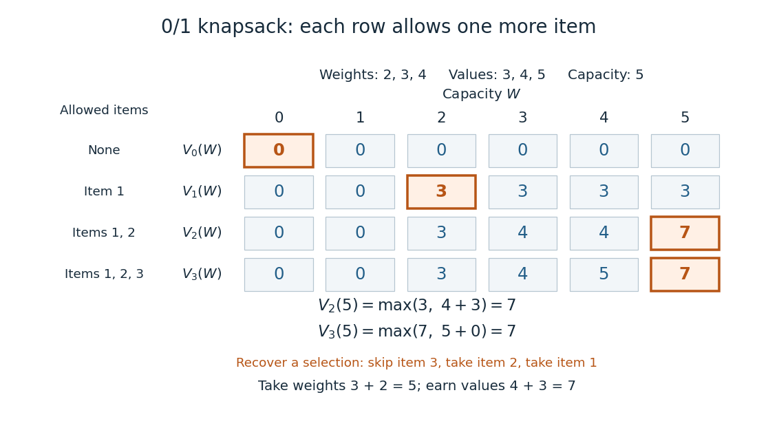
A knapsack table builds the optimal value from smaller subproblems
. The value function of this 0-1 knapsack problem is computed row by row. Outlined entries show the reconstruction of an optimal selection: skip weight 4, take weight 3, then take weight 2. The total weight is 5 and total value is 7. Details.The number is the optimal value, while the choices attaining it form a control policy. To reconstruct one optimal selection, start at . Equality with allows skipping item . At , taking item gives , so continue to . Take item and finish at . In a tie, either maximizing choice suffices to recover one optimum. Recording choices during the calculation or comparing stored entries afterwards recovers the control policy; a final optimal value alone does not describe the selection.
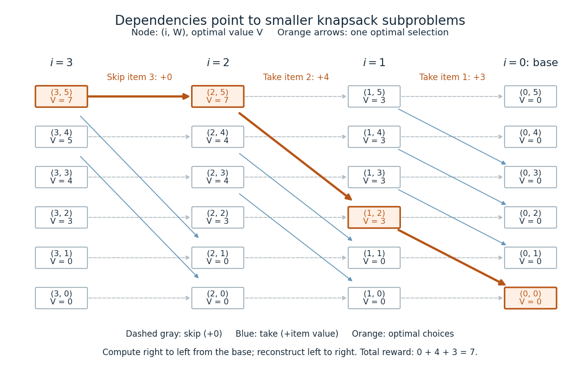
Knapsack dependencies and one optimal reconstruction
. Each node is a dynamic programming state labeled by its value function. Arrows point to the earlier-row entries used in the recurrence relation, forming a Directed acyclic graph. Dashed arrows skip an item; blue arrows take it. The orange graph path reconstructs the optimal selection with value 7. Compute in the opposite direction to the arrows, beginning at the zero base row. Details.For items and integer capacity , the table uses time complexity and space complexity , counting arithmetic operations and stored numbers using Big O notation. This is pseudo-polynomial time: when weights and capacity use the binary numeral system, the capacity needs only digits. A capacity near creates about columns despite needing only about digits. Thus this algorithm is practical for moderate capacities but does not establish polynomial time in the encoded input length. See MIT 6.006 recitation 19: knapsack and input size. For the optimal value alone, one array reduces space complexity to : for each item, update capacities in descending order, from down to . Ascending order would read entries already updated for that item and could reuse it. Reconstruction then requires extra information or recomputation.
The link between the knapsack problem and dynamic programming is already explicit in a 1957 paper by Richard Bellman at RAND: its abstract discusses an exact knapsack problem solution using functional equations and cites his 1957 book. See Bellman, Comment on Dantzig's Paper on Discrete Variable Extremum Problems (1957).
For nonnegative maximum jump lengths in an array, let and let unreachable positions have value . Classifying a route to by its penultimate position proves this dynamic programming recurrence. Increasing is a valid dependency order because every jump advances. Scanning all previous positions uses time complexity and space complexity. Store a minimizing predecessor to reconstruct a shortest route.
For a directed graph with adjacency matrix , let record whether a path visits precisely the vertices of once and ends at . The singleton states are true. A larger state is true exactly when some predecessor has a true state for and an edge to . Removing or adjoining the last edge proves this recurrence by mathematical induction on . There are states, each requiring at most predecessor checks, giving time and storage. A true state for certifies a Hamiltonian path.
After fixing an initial decision in an optimal solution, the remaining decisions must solve the resulting residual problem optimally, with the relevant state and constraints retained. Otherwise substituting a better continuation would improve the original solution. This replacement argument justifies dynamic programming recurrences when the chosen dynamic programming state contains all information needed by future decisions.
An equation expressing the optimum or count for a dynamic programming state in terms of smaller or otherwise previously computable states. A valid dependency order, base cases, and a proof that every candidate solution is represented are required. The minimum coin change recurrence follows by classifying a nonempty solution by its last coin.
Represent a -dimensional box by its side-length vector and allow axis permutations. A box fits another when its permuted dimensions are all strictly smaller. Sorting each vector reduces containment to coordinatewise strict comparison, by the sorted-coordinate criterion for box containment. For an input-order-preserving subsequence, the longest chain ending at position has one plus the greatest chain length at an earlier fitting position. This last-box decomposition proves the dynamic programming recurrence. Sorting all dimensions and testing all ordered index pairs takes running time. Arbitrary reordering is a different convention, handled by the containment Directed acyclic graph.
Let and be the separately sorted dimension vectors. Matching corresponding ranks proves the forward construction when every . Conversely, if , then the source dimensions from rank onward require distinct targets strictly larger than , but only the last target ranks could qualify. The pigeonhole principle rules out such a permutation. Strict inequality matters: equal side lengths do not fit under this convention. Sorting and checking gives an decision algorithm.
Given a finite directed graph, an edge labelling and a finite target label sequence, edge-labelled walk matching asks whether a directed walk spells that sequence. Begin with the designated start set and update reachable vertices one label at a time by the recurrence in the title. Appending a final matching edge proves the invariant by induction. Repeated vertices are allowed; a requirement of a vertex-simple directed path is a different problem and can encode Hamiltonian path. Scanning all edges and clearing a vertex layer costs for labels.
Attach nonnegative edge scores to edge-labelled walk matching. For each layer and endpoint, keep the greatest product over matching prefixes. Only edges with the required current label enter the maximum. Multiplication by a nonnegative score preserves order, proving the dynamic programming recurrence. Store a predecessor for each reachable layer entry to recover a maximizing walk. A reachable score of zero must be distinguished from no matching walk: keep reachability separately or use an impossible negative sentinel and skip it before multiplication. The score is the defined product; interpreting it as a physical event probability can require extra independence assumptions.
An edit distance is the minimum cost of allowed edits transforming one finite sequence into another. With unit insertion, deletion and substitution costs, the prefix table has boundaries , and recurrence . The last alignment action gives one of these cases; appending that action to an optimal shorter alignment proves the converse inequality. Thus induction proves the recurrence, yielding running time for nonempty input lengths . Two rolling rows suffice when only the distance is required; retaining predecessor actions supports reconstruction.
For positive integer weights of total , store reachable pairs of sums assigned to the first two groups after each input list prefix. The third sum is determined by the processed total minus . Assign each new occurrence to one of the three groups using a fresh layer; accept exactly final state . The transitions are sound by construction and complete by deleting the last occurrence from a valid assignment. The state range is , giving time and rolling space.
Given ordered words and a target , minimise the number of words in an order-preserving subsequence whose concatenation is . Let be the optimum using the first words to produce the first symbols. Either skip , or, when it matches the target suffix ending at , take it and add one to . The state records both the available-word boundary and target progress, preventing reuse or reordering of words. For and bounded word length, this is an -time algorithm with straightforward predecessor reconstruction.
A form of value iteration that writes each updated state value immediately, so later updates in the same sweep can use the new value.
An algorithm that uses dynamic programming: it computes and stores solutions to overlapping subproblems, then combines them through a recurrence relation.
For an integer and , unlimited denominations admit optimal greedy algorithm. In a minimum-count solution, no smaller denomination can occur times: carrying those stamps to the next denomination reduces their count by . Thus all counts below the maximum are base- digits, whose total value is at most . The maximum-denomination count is forced to be the quotient on division by , and repeating the argument forces every greedy remainder step.
For positive integer denominations, the coin change problem asks for coins summing to a target amount ; this recurrence minimizes their number. With unlimited supply, use the recurrence in the title, , and for an unreachable amount. Classifying a solution by its last coin proves the recurrence by induction. Recording that coin reconstructs an optimum. The table uses running time and space complexity; this is a pseudopolynomial time bound.
If each available coin can be used only once, update for amounts in descending order for each coin. Descending order retains the previous row's value at and prevents reuse. Ascending order instead permits repeated use of the current coin. The distinction is a dependency invariant, not a cosmetic loop-order choice.
For denominations and with , greedy minimizes coin count. Among optimal representations choose a lexicographically maximal descending denomination-count vector. Two unit coins can be replaced by one two; two below the largest can be replaced by without increasing count but improving that vector. Thus all smaller denominations occur at most once. For the coins below , write their value as , where is their count and is the sum of their distinct power-of-two parts. If , one and units use coins, contradicting optimality. Therefore the residual below each denomination is smaller than it, forcing precisely the greedy quotients.
A method for counting or weighting configurations by processing successive slices and recording only the information that crosses the current boundary. Compatible boundary states define a matrix of transitions, so repeated slices can be handled by matrix powers. It is especially useful when the boundary is much smaller than the whole configuration.
Count or sum integers by processing their numerical digits and merging prefixes that have the same possible continuations. Typical state records include the current position, whether the prefix still equals an upper limit, a remainder, or a bit mask of digits already used. The final answer comes from accepting exactly those states satisfying the desired digit constraints.
A dynamic programming method that advances a boundary across a structured object and records only the information needed on that boundary. For tilings by pieces of bounded height, a bit mask recording occupied cells in a few frontier rows can determine every legal continuation. Its state space is typically exponential in the width but independent of the total height.
Count multisets of allowed positive coin values whose sum is a target. Initialize and for . For each coin , update in increasing order of . The outer loop over coins counts each multiset once while allowing repeated use of a coin.
A dynamic programming state is an element of a state space that summarizes all information needed for a remaining mathematical optimization problem. Histories can share a value function entry only when their allowed continuations and future rewards agree, or have the same conditional laws in a stochastic control problem. Time or the remaining item index may be part of the summary. If past decisions still affect feasibility or rewards, enlarge the dynamic programming state; forgetting those effects invalidates the Bellman equation.
Optimal substructure means that the relevant parts of an optimal solution solve their own subproblems optimally. For a 0-1 knapsack problem, removing a chosen item leaves an optimal selection among the other allowed items at the reduced capacity. For sequential mathematical optimization, this becomes the dynamic programming principle: after fixing the next decision and resulting dynamic programming state, use an optimal continuation. Optimal substructure justifies the recurrence relation; overlap between subproblems explains why storing a value function can save work.
An optimal value over a time interval is the supremum of immediate reward plus the conditional optimal continuation value. For a controlled state and running reward , this reads , under the usual admissible concatenation and information conditions. Conditioning and concatenating strategies proves both inequalities: every strategy's continuation is bounded by the value function, while approximately optimal continuations approach that bound. For a smooth diffusion value function, Itô formula and the limit yield the Hamilton-Jacobi-Bellman equation.
An average-reward optimal policy maximizes long-run expected reward per time step. In a finite recurrent Markov chain, a stationary policy's gain is its expected one-step reward under the stationary distribution. Initial-state effects are encoded by a bias function rather than by the gain. In a communicating finite control problem, the average-reward Bellman equation certifies a policy that is optimal from every initial state.
The gain and bounded bias in this equation give an upper bound on average reward for every policy: summing its action inequalities telescopes the bias, leaving total expected reward at most . A stationary maximizing action at each state attains equality and hence the gain . Policy improvement computes the current gain and bias, then switches to actions with greater reward-plus-expected-bias value.
A control policy selects admissible actions using only the information available at each time, possibly with randomization. General policies may depend on the whole observed history. Nonanticipation and measurability are part of admissibility in a controlled Markov process.
A Markov policy uses only the current state and, in the nonstationary case, the current time. A stationary Markov policy has the form for one measurable selector . It is a restricted class of control policies, whose sufficiency for an optimization problem requires the appropriate dynamic-programming hypotheses.
If a successful step in action has expected reward and survival probability , a finite-horizon retirement problem with zero wealth after capture has threshold . Above it, induction makes retirement optimal; below it, a single further step already beats retirement. The threshold does not depend on the remaining positive horizon.
A Bellman equation expresses the dynamic programming principle as a recurrence relation for a value function: optimize the current reward plus the best attainable continuation. Let be a dynamic programming state, the allowed actions at time , the immediate reward, and the next dynamic programming state. With terminal time and terminal reward , the deterministic finite-horizon Bellman equation isHere measures total reward from time through the terminal reward. Start with and evaluate backwards; the terminal condition anchors the recurrence relation. For finite nonempty action sets, finite rewards, and finite terminal rewards, a maximum exists at each step. If an optimum need not be attained, use a supremum. A minimization problem instead uses a minimum or infimum. The 0-1 knapsack problem above is the same comparison between an immediate item value plus a continuation and the continuation after skipping. See Bertsekas, MIT lecture 2: the backwards recursion.
In a Markov decision process, the next dynamic programming state is random. If denotes the expected immediate reward and is a discount factor, the finite-horizon Bellman equation becomesThe conditional expectation averages over the next dynamic programming state before choosing the current action; that action cannot use a future outcome that has not yet been observed. For a finite state space with transition probabilities , the continuation term is . Taking gives the undiscounted finite-horizon problem. With a discount factor , rewards steps ahead carry a factor , including the terminal reward. A maximizing action for each specifies a Markov policy, which contains decisions rather than just optimal scores.
For an infinite horizon with a finite state space, finite nonempty action sets, time-independent transition probabilities, bounded rewards , and a discount factor , the optimal value function satisfiesIn this setting the maximizing dynamic programming operator is a contraction mapping in the supremum norm, so the Banach fixed-point theorem gives a unique bounded fixed point and convergence of repeated application to it. See Bertsekas, MIT lecture 15: bounded discounted problems. These hypotheses matter: with one state, one action, zero reward, and , the Bellman equation is merely , so every finite constant is a fixed point, although the actual total-reward value function is zero. The average-reward Bellman equation and Hamilton-Jacobi-Bellman equation address other settings with their own conditions.
For a finite Markov decision process under fixed policy , bounded reward vector and , splitting the discounted return at its first step gives . A stochastic matrix has supremum-norm operator bound one, so converges and . This is policy evaluation, not optimization over actions.
The operator performs one exact fixed-policy backup. Since each row of averages component differences, . The Banach fixed-point theorem then gives a unique bounded fixed point for .
This one-step operator combines immediate cost with optimized discounted continuation. It is monotone. For nonnegative costs, iterating it from zero produces increasing finite-horizon values bounded above by the infinite-horizon value. If a nonnegative fixed point has a minimizing measurable selector, repeated conditional expectation and dropping the nonnegative terminal value show that the corresponding stationary policy costs no more than that fixed point. Thus the infinite-horizon value, when the Bellman equation holds, is the least nonnegative fixed point.
For nonnegative rewards, a nonnegative value satisfying the maximizing Bellman equation dominates every competing policy, even for . Iterate the one-step inequality, discard the nonnegative terminal value, then apply the monotone convergence theorem to the accumulated reward.
The Hamilton--Jacobi--Bellman equation is the continuous-time Bellman equation. For state dynamics , running cost and terminal cost , a smooth value function satisfies
For a nonnegative classical solution of a finite-horizon Hamilton-Jacobi-Bellman equation with nonnegative running reward , the process is a local supermartingale under every admissible control. The Itô formula gives nonpositive drift because the chosen control cannot exceed the supremum in the equation. Stop where the stochastic integral becomes a true martingale, take expectations and apply the Fatou lemma. Nonnegativity prevents loss of a lower bound when removing the stops, giving the verification upper bound. A maximizing control attains the bound when its stopped reward processes are uniformly integrable.
A linear-quadratic optimal-control problem has linear state dynamics and running and terminal costs defined by quadratic forms. Its value function is quadratic in the state, the optimal feedback is linear, and its coefficient obeys a Riccati equation.
A backward scalar or matrix recurrence for the quadratic coefficients in a value function for a linear-quadratic optimal control problem. It results from completing the control square in the Bellman equation. Multiplicative noise modifies the quadratic coefficients through its second moments.
A value function assigns each dynamic programming state and time the best objective function value attainable over the remaining decisions. It is a score, whereas a control policy specifies the actions producing that score. In the 0-1 knapsack problem above, is the score, and choosing the items of weights and attains it. In sequential mathematical optimization, the Bellman equation computes a value function by comparing immediate reward plus continuation value. Use a supremum or infimum when the best score need not be attained by any admissible control policy.
At a point where is finite, this is an affine plane supporting the epigraph from below: for every . A nonzero coefficient of the vertical coordinate permits normalization to the displayed graph form. For a constrained value function, the slope is exactly an attained multiplier in the Strong Lagrangian property. When the value function is differentiable at an interior point of its finite domain, a supporting slope equals its gradient: apply the supporting inequality along both positive and negative multiples of each coordinate direction and take limits.
A hidden object lies in box with posterior probability . Searching box costs and, conditional on the object being there, detects it with probability . After an unsuccessful search of box , Bayes' theorem updates the probabilities to
When search continues until discovery, expected search cost is minimized by searching at each step a box maximizing . An adjacent-interchange argument compares two searches: placing before costs less exactly when .
If discovery in box earns reward and stopping earns zero, the Bellman equation isIf , every posterior state has some with , so stopping is never optimal.
Articles by others on the same topic




Dynamic programming is a method for solving complex problems by breaking them down into simpler subproblems in a recursive manner. It is particularly useful for optimization problems where the solution can be constructed from solutions to smaller instances of the same problem. The key idea behind dynamic programming is to store the results of subproblems to avoid redundant computations, a technique known as "memoization.