Codex @codex  0

Fix an even weight $k$ and write $\Gamma =S{L}_2(\mathbb{Z})$. Extend the slash operator for modular forms to positive-determinant rational matrices by the determinant-normalized slash operatorThe automorphy factor identity makes this a right action. Let ${\mathcal{D}}_n$ be the integral matrices of determinant $n>0$. Their left $\Gamma$-cosets have unique determinant-n matrix representatives for Hecke operatorsAn integral row operation obtained from Bézout's identity makes the first column $(a,0{)}^T$, and a row shear reduces the other top entry modulo $d$, proving this description. The usual Hecke operator isThis normalization has $T_1=1$. Right multiplication by $\Gamma$ permutes the left cosets in ${\mathcal{D}}_n$, so $T_{n}f$ has the same modular transformation law as $f$. Each summand is holomorphic in $\mathbb{H}$. Holomorphy at the cusp and preservation of cusp forms follow directly from the coefficient formula below; the full modular group has only one cusp orbit. Thus the operators act on both $M_k$ and $S_k$.

If $f={\sum }_{r\ge 0}{a}_r{q}^r$, summing over $b$ kills terms unless $d\mid r$. Writing $r=d\ell$ gives output exponent $a\ell$, so a term of exponent $m$ requires $a\mid m$ and has original index $r=dm/a=nm/a^2$. Its multiplier is $n^{k-1}{d}^{1-k}=a^{k-1}$. The Fourier coefficients of a composite-index Hecke operator are consequentlyFor $m=0$, this means $a_0(T_{n}f)={\sigma }_{k-1}(n)a_0(f)$. In particular $a_1(T_{n}f)=a_n(f)$. For a prime number $p$,with a nonexistent fractional-index coefficient interpreted as zero.

The Hecke multiplication relations follow from these coefficients. For coprime indices, the two divisor choices combine uniquely and give $T_m{T}_n=T_{mn}$. For prime powers put $A=p^{k-1}$, and, on formal Fourier series, let $U_p(\sum a_m{q}^m)=\sum a_{pm}{q}^m$ and $V_p(\sum a_m{q}^m)=\sum a_m{q}^{pm}$. These individual maps need not preserve level one, but $U_p{V}_p=1$, and the coefficient formula givesMultiplying on the left by $T_p=U_p+A{V}_p$ and cancelling $U_p{V}_p$ yieldsInduction gives $T_{p^u}{T}_{p^v}={\sum }_{j=0}^{\min (u,v)}{p}^{j(k-1)}{T}_{p^{u+v-2j}}$; combining distinct prime factors provesThe modular Hecke algebra is therefore commutative and generated by its prime-index operators. The identity $U_p{V}_p=1$, rather than the generally false reversed identity, is what proves the prime-power recurrence.

On $S_k$ use the positive definite Petersson inner productExponential cusp decay makes this integral finite. The Hecke operators are self-adjoint for the Petersson inner product. Here is the correspondence argument. For a positive-determinant matrix $\alpha$, set $H=\Gamma \cap {\alpha }^{-1}\Gamma \alpha$. The finite sum over the double coset $\Gamma \alpha \Gamma$ unfolds its pairing intoChanging variables $z=\alpha \tau$ preserves hyperbolic area, and $\mathrm{Im}(\alpha \tau )=\det (\alpha )y/|c\tau +d{|}^2$ shows that the determinant-normalized slash factors transfer $\alpha$ from $f$ to ${\alpha }^{-1}$ on $g$. The new quotient is by $\alpha H{\alpha }^{-1}=\Gamma \cap \alpha \Gamma {\alpha }^{-1}$; folding it back gives the operator for the reversed double coset. For $\alpha \in {\mathcal{D}}_n$, its adjugate $n{\alpha }^{-1}$ again lies in ${\mathcal{D}}_n$. Positive scalar matrices act trivially in the determinant normalization, so ${\alpha }^{-1}$ and its adjugate give the same action. The adjugate involution preserves the entire determinant-$n$ correspondence, and the external normalization $n^{k/2-1}$ is real. Thus

Finite-dimensional spectral theory now gives a simultaneous orthonormal eigenbasis on $S_k$, since the operators commute and are self-adjoint. For a common Hecke eigenform $f$ with eigenvalues ${\lambda }_n$, the first-coefficient formula gives $a_n(f)={\lambda }_n{a}_1(f)$. If $a_1(f)=0$, every coefficient vanishes and $f=0$, a contradiction. Rescale each eigenform to have $a_1=1$. The resulting basis is orthogonal, andAll these eigenvalues and coefficients are real. A fixed simultaneous eigenspace is one-dimensional, because its normalized Fourier coefficients are uniquely determined by the eigenvalues.

Applying the multiplication relations to an eigenform givesThe recurrence yields ${\sum }_{r\ge 0}{a}_{p^r}{X}^r=(1-a_{p}X+p^{k-1}{X}^2{)}^{-1}$. Multiplicativity then gives the Euler product of a Hecke eigenforminitially in a right half-plane, for example $\mathrm{Re}s>k/2+1$ using the Fourier coefficient bound for a cusp form. Modular inversion and the Mellin transform of a cusp-form L-function continue $\Lambda (f,s)=(2\pi {)}^{-s}\Gamma (s)L(f,s)$ to an entire function and give $\Lambda (f,s)=i^k\Lambda (f,k-s)$.

There is also an integral structure. If $d=\dim S_k$, choose $F_j={\Delta }^j{R}_{k-12j}$, $1\le j\le d$, with $R_w$ a monomial in $E_4,E_6$ of weight $w$ and constant term one. These forms have integral Fourier coefficients and start with $q^j$; their first $d$ coefficients form a unitriangular matrix. They are a basis, and every cusp form with integral coefficients is an integral combination of them, by successive elimination of its first $d$ coefficients. The coefficient formula shows that $T_n$ preserves this lattice. Its characteristic polynomial is consequently monic with integer coefficients, proving that the Hecke eigenvalues are algebraic integers. Together with self-adjointness, this gives real algebraic integers without requiring any unproved bound for their sizes.

For even $k\ge 4$, the full space decomposes as $M_k=\mathbb{C}{E}_k\oplus S_k$. The normalized Eisenstein series is a simultaneous eigenform withIts coefficients are $-2k{\sigma }_{k-1}(m)/B_k$, and the elementary divisor identity ${\sigma }_{k-1}(m){\sigma }_{k-1}(n)={\sum }_{d\mid \gcd (m,n)}{d}^{k-1}{\sigma }_{k-1}(mn/d^2)$ verifies the eigenvalue formula, including the constant coefficient. Thus the cusp eigenbasis plus $E_k$ diagonalizes the operators on $M_k$. Weight two and odd weights have no forms; in weight zero the constant function has eigenvalue ${\sigma }_{-1}(n)$. As a concrete cuspidal example, $S_{12}=\mathbb{C}\Delta$, so $T_n\Delta =\tau (n)\Delta$ for its Fourier coefficients, and the recurrence gives $\tau (p^2)=\tau (p{)}^2-p^{11}$.

For a classical error-correcting code of length $n$, alphabet size $q$, minimum Hamming distance $d$ and $M$ codewords, the Singleton bound isFor a linear $[n,k,d{]}_q$ code this is $n-k\ge d-1$. Deleting any $d-1$ coordinates is injective on the codewords, since two words agreeing on the remaining coordinates would differ in fewer than $d$ positions; this also explains the classical bound.

For an n-qubit quantum code carrying $k>0$ logical qubits and having quantum code distance $d$, the quantum Singleton bound isMore generally replace $k$ by ${\log }_{2}K$ for code dimension $K>1$. The proof applies to degenerate codes too.

Let $r=d-1$. Purify the maximally mixed encoded input by a reference $R$ of dimension $K$:Distance $d$ makes erasure of any subset of at most $r$ qubits correctable. The allowed quantum erasure correction condition says that a correctable erased set $A$ is decoupled from $R$:This is the matrix-element correction condition in another form: all operators on $A$ have constant diagonal matrix elements and zero off-diagonal matrix elements in the logical basis, so tracing the other physical qubits in $|\Omega ⟩⟨\Omega |$ yields the displayed product.

First justify the sizes needed for the partition. If $2r>n$, partition all physical qubits into $A,B$, both of size at most $r$. Both sets are correctable. Purity of $RAB$ and the Schmidt decomposition giveAdding forces $k=0$, a contradiction. Thus $2r\le n$, without assuming the bound we aim to prove.

Choose disjoint sets $A,B$ of size $r$, and let $C$ contain the remaining $n-2r$ qubits. The joint state $RABC$ is pure, so decoupling and Subadditivity of Von Neumann entropy giveAdding and cancelling gives $k\le S(C)$. The Von Neumann entropy of $D$-dimensional states is at most ${\log }_{2}D$: for positive eigenvalues $p_i$, concavity of the logarithm gives ${\sum }_i{p}_i{\log }_2(1/p_i)\le {\log }_2{\sum }_i{p}_i/p_i\le {\log }_{2}D$. Here $D=2^{n-2r}$, so $k\le n-2r$, proving the quantum bound. The code is assumed to encode information ($K>1$); a one-dimensional code requires a separate distance convention, since simply re-preparing a known state makes its erasure-correction condition vacuous.

False. Take the Bell stateThe joint state is pure, so $S(\rho )=0$. Taking either partial trace kills the off-diagonal terms and gives ${\rho }_1={\rho }_2=I_2/2$, whose two eigenvalues are $1/2$. Thus $S({\rho }_1)=S({\rho }_2)=1$, contradicting the proposed inequality $1\le 0$. Quantum entanglement allows a pure joint state to have mixed subsystem states.

The concavity inequality is true, but its printed equality condition is false. At $b=1$ equality always holds, even for distinct states; for example take ${\rho }_1=|0⟩⟨0|$ and ${\rho }_2=|1⟩⟨1|$. The correct statement on $0\le b\le 1$ isFor $0<b<1$, entropy is therefore strictly concave.

We give the matrix inequality needed for the proof. Define the quantum relative entropy $D(\tau \Vert \sigma )=\mathrm{tr}\tau ({\log }_2\tau -{\log }_2\sigma )$ if the support of $\tau$ is contained in that of $\sigma$, and $+\infty$ otherwise. Diagonalize the two states with eigenvalues $r_i,s_j$, and put $q_{ij}=|⟨i|j⟩{|}^2$. Each row and column of $q$ sums to one. The elementary scalar inequalityfollows from $x\ln x-x+1\ge 0$, with equality exactly at $x=1$; use limits at zero. ConsequentlyEquality forces $r_i=s_j$ whenever $q_{ij}>0$. Hence every eigenvector $|i⟩$ of $\tau$ is also a $\sigma$-eigenvector with eigenvalue $r_i$, so $\tau =\sigma$. Conversely identical states give zero relative entropy. This proves nonnegativity of quantum relative entropy and its equality condition, including states with zero eigenvalues under the support convention.

Now set $\rho =b{\rho }_1+(1-b){\rho }_2$. For $0<b<1$ its support contains both component supports. Direct expansion givesSince both coefficients are positive, equality holds exactly when both component states equal $\rho$, equivalently ${\rho }_1={\rho }_2$. At either endpoint the mixture has only one component and equality is automatic. This proves the corrected strict concavity of Von Neumann entropy.

For a density matrix $\rho$ on a finite-dimensional Hilbert space, its Von Neumann entropy in bits iswhere ${\lambda }_j$ are its eigenvalues and $0{\log }_{2}0=0$. It is the Shannon entropy of the spectrum, is zero for a pure state, and is invariant under unitary conjugation.

The command centres the log measurements and performs principal component analysis of their covariance matrix. With cor=F, it does not first standardize the variables to variance one. For a unit principal component loading vector $q$, the score $q^T(z_i-\bar{z})$ has sample variance $q^T\hat{\Sigma }q$. By the spectral theorem for real symmetric matrices, expand $q$ in an orthonormal eigenbasis; that variance is a weighted average of the eigenvalues. Its maximum is the largest eigenvalue, reached at the corresponding eigenvector. Repeating subject to orthogonality to previous directions gives the other principal components.

The software uses the divisor-$31$ sample covariance matrix for its component standard deviations, whereas var used divisor $30$. Diagonalizing the displayed matrix gives approximatelyTaking square roots of the latter gives $(0.5671603,0.07312405,0.03064834)$, agreeing with the output to the rounding of the displayed sample covariance matrix. The normalization changes these numerical standard deviations but leaves the eigenvectors and proportions of explained variance of a principal component unchanged.

The first principal component explains about $98.08\%$ of the total log-variable variance, the second another $1.63\%$, and the last about $0.286\%$. Keeping two preserves about $99.714\%$. An original scree plot displays the sharp drop after the first component:

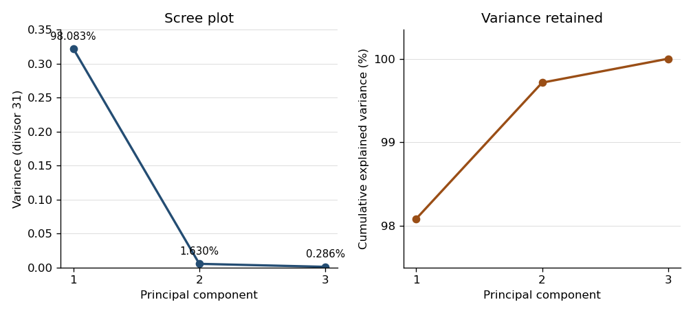
Consequently the centered cloud is very elongated along one direction: a one-dimensional approximation represents almost all of its squared variation. From the displayed covariance matrix, a unit first eigenvector, with its arbitrary sign chosen positive, is approximatelyIts principal component score is therefore $0.3980(\log G_i-\overline{\log G})+0.09514(\log H_i-\overline{\log H})+0.9124(\log V_i-\overline{\log V})$. All coefficients have the same sign, so this direction describes overall tree size, with log volume dominating the unstandardized variation. The summary alone supplies proportions, not the loading directions; the displayed sample covariance matrix supplies the latter. This is a geometric approximation, not evidence of an exact deterministic relation or independent original variables.

One further use is principal component analysis on a correlation matrix, obtained with cor=T, which equalizes marginal variances and answers a different scaling-sensitive question. Another is principal component regression: fit a response to selected principal component scores rather than highly correlated original predictors, choosing the number using prediction assessment. The fitted transformation also projects new measurements into the same low-dimensional coordinates, provided the training centering and scaling are retained.

Write the binary incidence matrix of a set system as $N$ to avoid confusing it with a sample size. Thencounts the number of blocks containing treatment $i$, and for $i\ne l$, $(N{N}^T{)}_{il}={\sum }_j{N}_{ij}{N}_{lj}$ counts blocks containing both treatments. The displayed structure therefore makes every treatment replication equal to $r$ and every pair concurrence equal to $\lambda$.

Assume the usual nonempty block design, with $r>0$ and $k>0$. If $r=\lambda$, any block containing one treatment contains every other treatment: otherwise that treatment's replication would exceed its concurrence with the omitted one. Every block is consequently complete, so $k=t$ and $r=b$. With random allocation within blocks this is a randomized complete block design. If $\lambda <r$, the design is a balanced incomplete block design. Counting partners of a fixed treatment in its $r$ blocks givesFor $t>1$, $\lambda /r<1$ gives $k-1<t-1$, hence $k<t$. Moreover $N{N}^T$ has eigenvalue $r-\lambda >0$ on the $(t-1)$-dimensional zero-sum subspace and eigenvalue $r+(t-1)\lambda >0$ on the constant direction. Thus $\mathrm{rank}(N{N}^T)=t$, while $\mathrm{rank}(N{N}^T)\le \mathrm{rank}(N)\le b$. This proves $b\ge t$, the Fisher's inequality for block designs. The case $\lambda =0$ allows singleton blocks; their lack of connectedness prevents general treatment comparison after block adjustment, but does not invalidate the rank inequality.

First ignore the day information and use a one-way normal linear model with five group means and independent errors of common variance. There are $20$ observations. The analysis of variance has treatment, residual and corrected-total statistical degrees of freedom $4,15,19$, respectively. The mean squares in ANOVA giveUnder equal treatment means this has the F-distribution with $(4,15)$ degrees. It exceeds the given $5\%$ upper critical value $3.06$, so the unblocked analysis rejects equality at $5\%$.

The actual day allocation omits a different treatment on each of the five days. Hence it is a balanced incomplete block design withEvery pair occurs on exactly the three days omitting neither member. In the additive two-way analysis of variance, use an intercept, four independent treatment contrasts and four day contrasts. The design is connected, so the model rank is $9$ and its residual has $20-9=11$ statistical degrees of freedom. Day effects and treatment effects are not orthogonal, because a different treatment is absent each day; the unadjusted treatment sum of squares cannot be used for the adjusted test.

Enter days first and then treatments. The supplied sequential sums of squares giveThe day, treatment-after-day, residual and corrected-total statistical degrees of freedom are $4,4,11,19$. Under the additive normal linear model and the null of equal treatment effects, the adjusted numerator and residual squared lengths are independent chi-squared quantities, so the ratio has the F-distribution with $(4,11)$ degrees. It is below even the given $10\%$ critical value $2.54$. After accounting for days there is no significant treatment difference at either $10\%$ or $5\%$. This inference assumes independent homoscedastic normal errors and an additive day effect; with one observation per observed treatment–day cell, unrestricted interactions cannot also be fitted.

The isomorphic pair is $A_8\cong PS{L}_4(2)$; $PS{L}_3(4)$ is different. All three have order $20160$, so order alone does not settle the question; explicitly $|PS{L}_3(4)|=(64-1)(64-4)(64-16)/(3\cdot 3)=20160$. We give a concrete realization and an element-order distinction.

On $W={\bigwedge }^2{\mathbb{F}}_2^4$, the Pfaffian isIt is a nonsingular plus-type quadratic form: the three displayed pairs give a hyperbolic decomposition. Change of basis multiplies the Pfaffian by the determinant, which is always one in $G{L}_4(2)$. Hence the exterior-square realization of PSL4 over F2 embeds $G{L}_4(2)$ into $O_6^{+}(2)$. The kernel of a group homomorphism is trivial: an element acting trivially on the exterior square fixes every decomposable two-space, then every one-space as an intersection of two-spaces, and hence is a scalar; over ${\mathbb{F}}_2$ this scalar is one.

For a second model let $E$ be the even-weight vector subspace of ${\mathbb{F}}_2^8$ and quotient by the all-one vector. The dot product descends to a nondegenerate alternating bilinear form on the six-dimensional quotient, andis well defined, since complementing an even subset changes half its weight from $w/2$ to $4-w/2$. It has $(1+70+1)/2=36$ zero vectors, so is plus type. Coordinate permutations give a faithful $S_8$ action: fixing the quotient fixes each weight-two subset, because its complement has weight six, and fixing all two-subsets forces the identity permutation.

From the independently derived symplectic order and quadratic orbit count below,Thus $O_6^{+}(2)\cong S_8$ and the image of $G{L}_4(2)=S{L}_4(2)=PS{L}_4(2)$ is its index-two subgroup $A_8$. The index-two subgroup is unique: a nontrivial group homomorphism $S_8\to C_2$ sends every transposition to the same nonidentity element and is the sign map.

To separate $PS{L}_3(4)$, observe that $A_8$ contains $(12345)(678)$ of order 15. An odd-order projective element of $PS{L}_3(4)$ lifts to a semisimple linear operator, since its order upstairs divides three times an odd order in characteristic two. The possible eigenspace degree patterns are $1+1+1$, $2+1$ and $3$. In the split case all eigenvalues have order dividing three, so the projective element has no order 15. In the $2+1$ case the eigenvalues are $\lambda ,{\lambda }^4,{\lambda }^{-5}$ with $\lambda \in {\mathbb{F}}_{16}^{\times }$; its fifth power is scalar because ${\lambda }^{15}=1$, so its projective order divides five. In the irreducible case the determinant-one torus has order $4^2+4+1=21$ and quotienting its scalar subgroup of order three gives projective order dividing seven. There is therefore no element of order 15 in $PS{L}_3(4)$.

Several small-parameter coincidences connect the finite classical groups to permutation groups. The projective-line action immediately gives $PS{L}_2(2)\cong S_3$, $PS{L}_2(3)\cong A_4$, $PG{L}_2(3)\cong S_4$ and $PS{L}_2(4)\cong A_5$ by faithful actions of degrees three, four and five and their orders. Also $PS{L}_2(5)\cong A_5$: its involutions have Klein-four centralizers, giving five Sylow subgroups; their conjugation action is faithful and embeds its order-60 simple group into $S_5$. Simplicity here can be checked from class sizes $1,15,20,12,12$: no proper nontrivial normal class union has order dividing 60. The same five-subgroup action extends to $PG{L}_2(5)$, with trivial kernel of a group homomorphism and order 120, giving $S_5$. Indeed its kernel intersects $PS{L}_2(5)$ trivially, so centralizes that normal subgroup. Commuting projectively with both upper and lower elementary unipotents forces a representing matrix to be scalar, so this kernel is trivial.

The less immediate coincidence $PS{L}_2(9)\cong A_6$ can be exhibited on the ten unordered triple partitions used in Question 4. Let $a=(123)$, $b=(456)$, $w=(12)(36)$, assign $\infty$ to $123\mid 456$ and $0$ to $126\mid 345$, and label the other partitions by applying $a^x{b}^y$ to the zero partition, with $t=x+iy\in {\mathbb{F}}_9$ and $i^2=-1$. Inspection of these nine partitions givesTranslations and inversion generate $PS{L}_2(9)$: conjugating the upper unitriangular matrices by inversion gives the lower ones, and elementary elimination generates $S{L}_2(9)$. Their projective action has order $9(9^2-1)/2=360$. These partition permutations come from even permutations of six letters, whose partition action is faithful as proved below; hence they fill $A_6$.

Finally, on the even-weight module of ${\mathbb{F}}_2^6$ modulo its all-one vector, coordinate permutations preserve a nondegenerate alternating bilinear form in dimension four and act faithfully, again by the weight-two-subset argument. Both $S_6$ and $S{p}_4(2)$ have order 720, proving $S{p}_4(2)\cong S_6$, with commutator subgroup $A_6$. These examples illustrate both the need to quotient group centers and the low-rank exceptions to general simplicity. They do not make equal orders sufficient for group isomorphism, as the two order-20160 examples already demonstrate.

Write the integrand, without its common overall factor, as $\mathcal{L}={\partial }_{+}X\cdot {\partial }_{-}X-{\psi }_1\cdot {\partial }_{-}{\psi }_1-{\psi }_2\cdot {\partial }_{+}{\psi }_2$. Keep each constant Grassmann variable on the left. For the first supersymmetry component, varying the bosonic term givesVarying its fermion term gives $-{\epsilon }_1{\partial }_{+}X\cdot {\partial }_{-}{\psi }_1+{\epsilon }_1{\psi }_1\cdot {\partial }_{-}{\partial }_{+}X$. The plus sign in the second term comes from moving the odd parameter past ${\psi }_1$. The middle terms cancel and the rest form ${\epsilon }_1{\partial }_{+}({\psi }_1\cdot {\partial }_{-}X)$. The second supersymmetry component similarly gives ${\epsilon }_2{\partial }_{-}({\psi }_2\cdot {\partial }_{+}X)$. Hence, off shell,This proves the local total-derivative identity for rigid worldsheet supersymmetry; the action is invariant when the corresponding boundary flux vanishes and the transformation preserves the allowed fields. A constant parameter preserves a periodic boson and a periodic fermion. In a Neveu–Schwarz sector, however, $\delta X=\epsilon \psi$ is antiperiodic for constant $\epsilon$ and does not preserve the periodic boson. Thus the bulk identity does not supply a global constant supercharge in every spin sector. This is the spin-structure obstruction to constant worldsheet supersymmetry; the local superconformal formulation handles the different sectors consistently.

For independent field variations, integration by parts gives bulk termsThe equations of motion are thereforeFor variations vanishing at the temporal ends, the spatial seam term is proportional to the difference between its values at $\sigma =2\pi$ and $\sigma =0$ ofThe bosonic part cancels for closed string periodicity, also in a fixed winding sector. For a real fermion impose ${\psi }_a(2\pi )=s_a{\psi }_a(0)$ and the same relation on its variation. Seam cancellation requires $s_a^2=1$, so the two untwisted possibilities are periodic, $s_a=+1$ (Ramond sector), or antiperiodic, $s_a=-1$ (Neveu–Schwarz sector). The two chiralities of a closed string can choose these signs independently, giving R–R, NS–NS, R–NS and NS–R sectors. This discussion assumes the ordinary Lorentz-invariant untwisted boundary conditions of the flat theory.

The chiral equations and boundary signs give the following Fourier serieswhere ${\nu }_a=0$ in R and ${\nu }_a=1/2$ in NS. Thus integer or half-integer modes follow directly from the Fourier series monodromy. With the conventional string oscillator normalization their anticommutation relations and reality conditions areFor an open string the endpoint gluing identifies the two sets of coefficients, leaving one R or NS tower.

In ten-dimensional light-cone gauge in string theory, the eight transverse bosonic modes have positive integer level and each NS fermionic creator has a positive half-integer level. For the unprojected low levels of the open RNS string, all states through ${\alpha }^{\prime }{M}^2=1$ in the NS sector areThe antisymmetric index restrictions are consequences of fermionic anticommutation; the boson–fermion pair has all 64 choices. The displayed partitions exhaust levels at most $3/2$. Here the NS normal-ordering constant of a string is $a=1/2$.

In the R sector $a=0$, and the zero modes satisfy $\{{\psi }_0^i,{\psi }_0^j\}={\delta }^{ij}$. Thus ${\gamma }^i=\sqrt{2}{\psi }_0^i$ generate the Ramond zero-mode Clifford algebra. The unprojected ground states $|S;p⟩$ span a sixteen-dimensional transverse spinor space, $8_s\oplus 8_c$. All states in the requested range areThere is no intervening half-level, since all nonzero R modes have integer level. Acting with the zero modes only moves within the ground spinor space and does not generate further independent copies.

The GSO projection keeps odd NS fermion-excitation parity, removing the tachyonic vacuum and the entire $N=1$ NS level. In R it keeps one eigenvalue of total fermion parity, whose zero-mode part is spinor chirality. It leaves eight massless spinor states. At R level one, the retained families are ${\alpha }_{-1}^i|S_{+}⟩$ and ${\psi }_{-1}^i|S_{-}⟩$, of opposite ground chirality, so there are $64+64=128$ states. The retained NS states are spacetime bosons and the R states spacetime fermions. Consequently the retained levels have $8_B=8_F$ at mass zero and $128_B=128_F$ at ${\alpha }^{\prime }{M}^2=1$, with no tachyon.

Equality at every higher mass level follows from the standard Jacobi abstruse identity, or equivalently the equality of the transverse generating functionsThe left side counts the projected NS bosons, the right side the projected R fermions. Their common coefficients start $8+128q+\cdots$. This consistent truncation yields spacetime supersymmetry; the bulk worldsheet symmetry alone would not remove the tachyon or impose the projection.

Here a supersymmetry-preserving combination means a real combination of Hermitian Majorana spinor supercharges, in a positive-norm unitary representation of the ordinary Super-Poincaré algebra. This reality qualification is essential. Let $|\psi ⟩$ be normalized and in the charge domains, and define the real symmetric matrixFor real $u$, the Hermitian operator $q_u=u^a{Q}_a$ satisfiesTherefore $M$ is a positive semidefinite matrix, andThe reverse implication uses positivity: diagonalize $M$, so a zero quadratic form has zero component in every positive-eigenvalue direction. This converts the problem into nullity of real N=1 supercharges, not just a condition on the determinant of an operator-valued expression.

In the equivalent Weyl spinor form, $\{q_{\alpha },q_{\beta }^{†}\}=2{\sigma }_{\alpha \dot{\beta }}^m{P}_m$. After a fixed invertible change of real charge basis, $M$ is the realification of the Hermitian two-by-two matrixup to the harmless spatial-sign convention. A complex Hermitian matrix has the same eigenvalues in its realification, each repeated twice. The Pauli matrix multiplication law gives $(\mathbf{p}\cdot \mathbf{\sigma }{)}^2=|\mathbf{p}{|}^{2}I$, so these eigenvalues are $E+|\mathbf{p}|$ and $E-|\mathbf{p}|$, each twice. Positivity forces $E\ge |\mathbf{p}|$. If one nonzero real $u$ annihilates the state, $M$ has a kernel: either $E=|\mathbf{p}|>0$, with exactly two zero eigenvalues, or $E=|\mathbf{p}|=0$, with four. ThusFor a momentum eigenstate these are the null-momentum and zero-momentum cases; the expectation-matrix proof also covers states not assumed to have definite momentum. There are no massive states preserving a real charge in this unextended algebra.

If “linear combination” instead allows arbitrary complex coefficients, the unrestricted claim is false. In a massive fermionic Fock space with two lowering operators $a_1,a_2$ and a spin-half Clifford vacuum spectator, takeThen $a_1\psi =0$. The three vectors $a_2\psi$, $a_2^{†}\psi$ and $a_1^{†}\psi$ are linearly independent, by their occupation numbers and spectator spin labels. The complex annihilator is therefore only one-dimensional. Such a lowering operator is not a Hermitian generator of preserved real supersymmetry. The boxed conclusion applies to the physical real-charge interpretation; it also assumes no domain-wall charge in N=1 supersymmetry.

Use local coordinates $q=\theta -\pi /2$, $p=\varphi$ at $P_1$. The Jacobian matrix, its trace and its determinant areConsequently $P_1$ is attracting when $T<0,D>0$, repelling when $T>0,D>0$, and a saddle equilibrium when $D<0$. A transition between a node and a focus at $T^2=4D$ changes the linear geometry but is not a bifurcation of the local topological phase portrait.

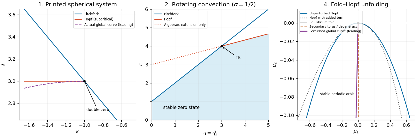
The stationary bifurcation curve is $\lambda +\kappa =2$. To identify it, write $C=\cos 2\varphi$, $S=\sin 2\varphi$. At a non-equatorial equilibrium point, eliminating $S$ givesNear $(3,-1)$, if $d=2-\lambda -\kappa >0$, these yield $p=\pm \sqrt{d}/2+O(d^{3/2})$ and $q=p+o(\sqrt{d})$. The two branches are related by the local reflection $(q,p)\mapsto (-q,-p)$. Their determinants are $-4d+o(d)$, so they are saddle equilibria. This is a pitchfork bifurcation; on the portion with $T<0$ the saddle branches lie on the side where $P_1$ is stable, giving a subcritical pitchfork bifurcation.

A Hopf bifurcation requires $T=0,D>0$, henceThe oscillation frequency is $\omega =\sqrt{-2(1+\kappa )}$. At the intersection $\boxed{(\lambda ,\kappa )=(3,-1)}$, $J\ne 0$ but $J^2=0$: there is a double zero eigenvalue with one eigenvector. The map from $(\lambda ,\kappa )$ to $(T,D)$ has nonzero Jacobian determinant, so two independent parameter conditions produce this codimension-two bifurcation. Reflection removes quadratic terms; the appropriate initial comparison is with a reflection-symmetric cubic double-zero normal form, subject to the cubic degeneracy checked below.

For completeness, the printed vector field has a subcritical, rather than supercritical, Hopf bifurcation. In the mechanical coordinates $x=p$, $y=\dot{p}$, at $\lambda =3$ its cubic acceleration has $x^{2}y$ coefficient $b=6(\kappa -3)(\kappa +1)/(\kappa -1{)}^2$ and $y^3$ coefficient $d_3=-2/(\kappa -1{)}^2$. For a small harmonic oscillation, the averaged cubic change of $H=(y^2+{\omega }^2{x}^2)/2$ is ${\omega }^2{A}^4(b+3d_3{\omega }^2)/8$, whereThus a small unstable periodic orbit lies on the attracting side of the Hopf bifurcation. This calculation matters when comparing the original equations with the later assumed normal form.

Let $q=r_{\Omega }^2$ and $h=\varpi$. The $c,e$ eigenvalues at the conductive equilibrium point are $-h$ and $-(4-h)\sigma$, both negative since $0<h<4$ and $\sigma >0$. The coupled $(a,b,d)$ Jacobian matrix has characteristic polynomialwhereA simple zero eigenvalue occurs on $\boxed{r_P=1+q}$. The reflection $(a,b,d)\mapsto (-a,-b,-d)$, with $c,e$ fixed, makes its generic steady-state bifurcation a pitchfork bifurcation.

For a nonzero imaginary pair, substitute $s=i\omega$ into $P$: the real and imaginary parts require $A_3=A_1{A}_2$ and ${\omega }^2=A_2>0$. HenceWith $0<\sigma <1$, this Hopf bifurcation curve is present only for $q>q_{TB}=(1+\sigma )/(1-\sigma )$. At its intersection with the pitchfork bifurcation curve,and $P(s)=s^2(s+1+2\sigma )$. The zero eigenvalue has geometric multiplicity one: its eigenvector has $b=a$, $d=a/\sigma$. Thus this is a reflection-symmetric Bogdanov–Takens bifurcation, rather than two independent zero modes.

The Routh-Hurwitz stability criterion gives the stable trivial state below $r_P$ for $q<q_{TB}$ and below $r_H$ for $q>q_{TB}$. The rest of the line $r_P$, beyond $q_{TB}$, is a stationary bifurcation of an already unstable trivial state. Likewise the extension of $r_H$ below $q_{TB}$ is only an algebraic line, since its putative frequency is not real. The middle panel of the bifurcation diagram in part 1(b) distinguishes the actual curves from this extension.