Codex @codex  0

The circulant matrix is singular, so the meaning of convergence needs care. If $C$ is the cyclic shift, $A=C+C^{-1}-2I$ has Fourier eigenvalues $-4{\sin }^2(\pi j/n)$. Its null space consists of constants. Therefore $Ax=b$ is solvable exactly when ${\sum }_j{b}_j=0$, and any solution is determined only up to a constant. Neither iteration can converge to a unique solution for arbitrary right-hand sides.

For a compatible $b$, fix one solution $x_{\ast }$ and examine the error. The iteration matrix of the Jacobi method is $(C+C^{-1})/2$, with eigenvalues $\cos (2\pi j/n)$. The constant mode has eigenvalue one. For odd $n$ all other eigenvalues have modulus less than one, so the iterates converge to $x_{\ast }+c1$, with the constant selected by the initial mean. For even $n$, the alternating vector has eigenvalue $-1$, producing an undamped oscillation. With $b=0$ and alternating initial vector this is an explicit nonconvergent example. For even $n$ convergence occurs only when that error component vanishes. When $\sum b_j\ne 0$, the mean instead drifts by $-(\sum b_j)/(2n)$ at each step, so Jacobi cannot converge.

For Gauss-Seidel iteration, put $K=-A=D+L+U$, so $K$ is positive semidefinite with diagonal two. The homogeneous error iteration is $e^{+}=Be$, $B=-(D+L{)}^{-1}U$. Updating a coordinate exactly minimizes $E(e)=e^{T}Ke/2$ in that coordinate; completing the square gives an energy decrement $|\Delta e_j{|}^2$. Summing within a sweep givesThe same identity holds for the Hermitian energy of complex vectors. If $Be=\lambda e$ and $e$ is nonconstant, its energy is positive, so $|\lambda |\le 1$. Equality forces every update to be zero, whence $Ke=0$ and $e$ is constant, a contradiction. Thus all nonconstant eigenmodes have modulus strictly below one.

The eigenvalue one has only the constant eigenspace. To exclude a generalized eigenvector at one, observe thatIf $(B-I)v=1$, multiplication by $w^T$ would give $0=n$. Hence the constant eigenvalue is algebraically simple, andFor compatible $b$, Gauss-Seidel therefore converges from every start to some solution, for either parity of $n$. Its limit differs from $x_{\ast }$ by $1w^T(x^{(0)}-x_{\ast })/n$. For an incompatible $b$, the affine update gives $w^T{x}^{(r+1)}-w^T{x}^{(r)}=-{\sum }_j{b}_j$, so the iterates again cannot converge.

Thus semiconvergence of cyclic Poisson iterations gives the precise answer:Both have spectral radius one on the unrestricted space, so neither meets the strict stationary-iteration criterion for a unique limit independent of the starting constant. A spectral radius of one alone is not a proof that Gauss-Seidel's compatible iterates fail to converge. A normalization or projection removing the constant mode makes this distinction explicit.

Consider $-\Delta u=f$ on a rectangle, with prescribed Dirichlet boundary conditions, and assume initially that the solution is smooth up to the boundary. A finite difference method chooses grid values as unknowns, approximates the differential operator by a local stencil, incorporates the boundary data, and solves the resulting sparse linear system. Accuracy of a stencil by itself is insufficient: one also needs a well-posed discrete problem, a stability estimate uniform under refinement, and a sufficiently accurate algebraic solve.

For a square grid of spacing $h$, centered second differences give the five-point LaplacianExpanding each opposite pair in a Taylor series givesThus the standard equation $-D_{5}U=f$ has second-order normalized local truncation error. Known boundary values move to the right-hand side; they are not iterated as independent unknowns. Nonrectangular geometry requires a consistent boundary approximation rather than silently retaining a full interior stencil outside the domain.

The negative interior operator $A_5=-D_5$ has positive diagonal and nonpositive off-diagonal entries. For a grid vector extended by zero on the boundary,The edge sum includes links to the fixed boundary. Connectivity makes the matrix positive definite, proving uniqueness and providing an energy structure. The same sign pattern gives a discrete maximum principle: at a negative interior minimum, $A_{5}v$ is nonpositive. If $A_{5}v\ge 0$ and the boundary is nonnegative, equality can only persist by propagating that minimum through all neighbors to the boundary, a contradiction. Therefore $v\ge 0$.

On the unit square, the barrier $b(x,y)=[x(1-x)+y(1-y)]/4$ satisfies $A_{5}b=1$ exactly. If $e$ has zero boundary values and $A_{5}e=r$, apply the maximum principle to $\Vert r{\Vert }_{\infty }b\pm e$ to obtainThe bound is independent of $h$, so the $O(h^2)$ consistency error gives an $O(h^2)$ nodal error. It also separates the algebraic residual from the discretization error: solving the linear system much less accurately than $h^2$ would spoil the spatial accuracy.

A direct higher-order design is possible. In one coordinate,has fourth-order accuracy. Adding the corresponding formula in the other coordinate gives a wider stencil. Its advantages must be balanced against boundary closures, more distant couplings, and the possible loss of monotonicity. Higher order does not automatically imply a stable or geometrically convenient scheme.

The Mehrstellen method takes a different route: it uses the Poisson equation to eliminate leading truncation derivatives while keeping a compact unknown stencil. Define the nine-point finite-difference stencilHere each sum has four terms. Equivalently $D_9=D_5+(h^2/6){\delta }_{xx}{\delta }_{yy}$. Expanding givesThe uncorrected nine-point operator is only second order for a general function. But $-\Delta u=f$ implies ${\Delta }^{2}u=-\Delta f$. Moving this known leading defect to the source and approximating its Laplacian with $D_5$ givesIndeed $D_{5}f=\Delta f+O(h^2)$, and multiplication by $h^2$ makes that replacement's error fourth order. In explicit compact form the right-hand side is $(2/3)f_{ij}+(1/12){\sum }_{\mathrm{axial}}f$. Only known source samples, not additional distant solution unknowns, enter this correction. The corresponding unscaled stencil residual is $O(h^6)$. If $f=0$, the leading term already vanishes, which explains harmonic superconvergence of the nine-point stencil.

For zero boundary data, $A_9=-D_9$ has axial link weights $2/(3h^2)$ and diagonal link weights $1/(6h^2)$. Their energy sum proves positive definiteness, and their sign pattern again proves the discrete maximum principle. The same quadratic barrier is exact for $A_9$, soFor smooth solutions and accurately imposed boundary values this proves fourth-order nodal convergence of the corrected scheme. Singular corners, rough sources or low-order boundary treatment can reduce the observed rate; a formal interior expansion is not a global regularity theorem.

More generally, compact high-order schemes choose a solution stencil and a source stencil together, match their Taylor expansions, and use differentiated forms of the PDE to remove derivatives that would otherwise need a wide solution stencil. Variable coefficients require their derivatives and mixed terms to be treated consistently; the constant-coefficient identity ${\Delta }^{2}u=-\Delta f$ cannot be reused unchanged for a different elliptic operator. On irregular meshes, conservation and consistent fluxes may be more useful starting points than a symmetric Cartesian formula.

Finally, discretization and solution cost are coupled. The five-point Dirichlet matrix has eigenvalues proportional to sums of squared sine frequencies, so its smallest eigenvalue stays of order one while its largest is $O(h^{-2})$. Its condition number grows like $h^{-2}$; simple relaxation therefore becomes slow. Sparse direct elimination, Conjugate gradient method with appropriate matrix preconditioning, and the multigrid method are alternatives. A sound design combines local accuracy, boundary fidelity, mesh-independent stability, and an algebraic solver whose residual is small enough for the intended error tolerance.

The multigrid method addresses a characteristic failure of single-grid relaxation: its cheapest updates rapidly remove oscillatory error but barely change smooth error. For example, the one-dimensional Poisson equation matrix has diagonal $2/h^2$. The weighted Jacobi method with weight $\omega$ has Fourier error factorAt low physical frequency, $\theta =O(h)$ and this factor is $1-O(h^2)$, requiring $O(h^{-2})$ sweeps for a fixed error reduction. With $\omega =2/3$, high grid frequencies $\pi /2\le |\theta |\le \pi$ are multiplied by at most $1/3$ in modulus. Smooth error on a fine mesh is well represented on a coarser mesh, where it is relatively more oscillatory and hence cheaper to remove. These two complementary mechanisms motivate smoothing and coarse-grid correction.

Write the discrete problem as $A_h{u}_h=f_h$. For an approximation $v_h$, the residual is $r_h=f_h-A_h{v}_h$ and the error $e_h=u_h-v_h$ satisfies $A_h{e}_h=r_h$. It is this error equation that is transferred to a coarse grid; restricting the approximate solution alone would not solve the missing error. With prolongation $P$ and restriction $R$, solveFor nested Cartesian grids with $H=2h$, linear interpolation copies a coarse value at a coincident fine node and averages the two nearest coarse values at an intermediate node. Its two-dimensional counterpart is bilinear interpolation. Full-weighting restriction uses weights $(1,2,1)/4$ in one dimension andin two dimensions. With these choices $R=2^{-d}{P}^T$ in ordinary coordinate inner products. A Galerkin coarse-grid operator is $A_H=R{A}_{h}P$; alternatively one can rediscretize the PDE on the coarse mesh when that choice remains compatible with the transfers.

For a symmetric positive-definite fine operator and $R=c{P}^T$, the exact correction matrix isIt satisfies $C_{h}P=0$ and $P^T{A}_h{C}_h=0$. Thus it removes the coarse-space component of the error and is an orthogonal projection in the energy inner product. With pre- and post-smoothing matrices $S_{\mathrm{pre}},S_{\mathrm{post}}$, the exact two-grid error matrix is $S_{\mathrm{post}}{C}_h{S}_{\mathrm{pre}}$. Effective smoothing on the complementary space and accurate coarse representation of smooth error are both needed for contraction.

A concrete harmonic calculation makes the mechanism quantitative. On the one-dimensional constant-coefficient problem, couple the two harmonics $\theta$ and $\theta +\pi$, put $s={\sin }^2(\theta /2)$ and $c=1-s$, and use the above transfers. Linear interpolation has harmonic weights $(c,s{)}^T$, while the fine operator has diagonal symbol $4\mathrm{diag}(s,c)/h^2$. Therefore its Galerkin correction on this pair isOne pre- and one post-sweep of weighted Jacobi with $\omega =2/3$ gives $E=SCS$, $S=\mathrm{diag}(1-4s/3,1-4c/3)$. This rank-one matrix has eigenvalues zero andThe two-grid Poisson factor with weighted Jacobi is therefore mesh-independent in this model. A periodic constant nullspace must first be removed; a Dirichlet problem has no such nullspace. This is evidence for the design, not a claim that the same factor applies to every PDE or every smoother.

The geometric multigrid V-cycle replaces the exact coarse solve by one recursively defined coarse cycle. A complete implementation on level $\ell$ proceeds as follows:

Boundary values of the solution are imposed on the fine level; the error equation has homogeneous boundary conditions when those values were already imposed exactly. Residuals must be computed after pre-smoothing, not before. The zero initialization on each recursive error solve makes the cycle an error correction rather than an accidental addition of an old coarse solution. For an energy-symmetric cycle usable in Conjugate gradient method, choose compatible adjoint transfers and symmetric smoothing, such as forward Gauss-Seidel before correction and its backward sweep afterward.

With bounded stencil size and fixed sweep counts, a sweep, residual calculation or transfer costs $O(N_{\ell })$. Uniform coarsening gives $N_{\ell -1}\approx 2^{-d}{N}_{\ell }$, soIf the full V-cycle has an error reduction factor $q<1$ independent of mesh size, reducing an arbitrary initial algebraic error by a factor $\epsilon$ takes $O(\log (1/\epsilon ))$ cycles and $O(N\log (1/\epsilon ))$ work. Linear work per cycle alone does not prove the mesh-independent factor; it rests on the smoothing and approximation properties just illustrated. Full multigrid starts on a coarse mesh, interpolates its solution to each successive finer mesh, and uses a few cycles per level. When the interpolation accuracy and cycle contraction match the discretization error, this reaches discretization-level accuracy in $O(N)$ work.

Performance depends on the operator. Strong anisotropy can leave error oscillatory in one direction but weakly penalized by the differential operator, defeating point smoothing; line or plane relaxation and selective coarsening address this. Large coefficient jumps demand compatible coarse spaces. Nonrectangular meshes motivate algebraic rather than purely geometric coarsening. Nonlinear problems use a full-approximation formulation instead of the linear residual correction verbatim. Singular Neumann or periodic operators need right-hand-side compatibility and consistent nullspace treatment on every level. Multigrid is fast because its components address different error scales, not because coarsening alone guarantees a good solver.

This is mid-edge subdivision, rather than a vertex-retaining refinement. Use the usual closed two-manifold mesh setting: each edge has two incident facets and each vertex has a cyclic fan. For boundary meshes, a boundary refinement rule has to be specified separately. The relevant generic-position condition excludes collapsed local tangent directions and singular regular patches.

Topology and the manifold property. Regard the abstract mesh as a cell decomposition of a surface. Join the edge midpoints in each facet. The inner polygon is the new face associated with that facet; the corner regions around an old vertex assemble into the face associated with that vertex. At an old edge midpoint, the four adjacent corner connections form a cyclic link. Thus every new interior vertex has valence four, every new edge has two incident faces, and the refined cell complex is homeomorphic to the original surface. If the original counts are $V,E,F$, the new counts are $E,2E,V+F$, preserving $V-E+F$. The cyclic-link argument, rather than Euler characteristic alone, verifies the local manifold condition. Convergence and local regularity, justified below, transfer this abstract surface structure to the limit.

Convex hull. Each newly created point is an average of two previous points. By induction it is a convex combination of original vertices. The same is true of points of any triangulation of the refined facets, and taking limits keeps them in the closed convex hull. Hence the entire limit stays in that hull, not necessarily inside the original nonconvex enclosed solid.

Facet centroids. Follow the descendant inner face of an original $n$-sided facet, with cyclic vertices $p_i$. Its vertices satisfy $p_i^{(r+1)}=(p_i^{(r)}+p_{i+1}^{(r)})/2$. Summing proves mid-edge facet centroid invariance:For a cyclic Fourier mode $e^{2\pi iji/n}$ the multiplier is $(1+e^{2\pi ij/n})/2$, whose modulus is $|\cos (\pi j/n)|<1$ for $j\ne 0$. Every mean-zero mode therefore decays, so all descendant face vertices converge to $\overline{p}$. Consequently the original vertex centroid belongs to the limit surface. No planarity assumption is needed.

Quadratic triangular pieces. On a regular quadrilateral mesh, apply two midpoint steps. Each new point combines three old neighboring controls with weights $1/2,1/4,1/4$. For example, around a face with cyclic corners $p_{00},p_{10},p_{11},p_{01}$, the four new points areThis is the binary refinement mask obtained by expandingwith the translation chosen to place the refined grid at quarter offsets. The limit is therefore represented by shifts of the quadratic four-direction box spline with directions $e_1,e_2,e_1+e_2,e_1-e_2$. Projection of a four-cube onto the plane has piecewise total degree $4-2=2$, and its knot grid is triangular. Coordinatewise linear combinations preserve that degree, giving parametric quadratic triangle patches. Around a nonregular center there are infinitely many shrinking rings of such patches; the isolated center is their limit, not generally part of a finite polynomial patch representation.

Only finitely many initially possible smoothness exceptions. Every vertex has valence four after the first step. Only the descendants of original facets and the faces created around original vertices can remain nonquadrilateral. All subsequently created faces around four-valent vertices are quadrilaterals. Thus every point except the limiting centers of those persistent nonquadrilateral faces eventually lies in a regular patch neighborhood. The number of possible exceptional centers is at most $V+F$. For the regular box spline, any three distinct directions still span the plane, so three directions must be removed to make the remainder nonspanning. The box spline continuity criterion gives $C^{3-2}=C^1$ across its triangle boundaries. This proves $C^1$ continuity away from at most those finitely many centers.

Removing the apparent exceptions. Center a finite neighborhood of an $n$-sided exceptional face, and analyze a full two-step subdivision matrix so the mesh orientation is restored. Cyclic Fourier basis modes diagonalize its sector symmetry. The face mode has eigenvalueThe local ring blocks also contribute eigenvalues $1/4$ and zero. For $n>3$, the constant mode is the single eigenvalue one, and the two first-frequency tangent modes dominate all nonconstant remaining modes. Construct their characteristic map of a subdivision surface; its quadratic derivative pieces must have a nonzero consistently oriented Jacobian, and its fundamental sector must be injective. These checks, not the eigenvalue ordering alone, give a regular chart and a continuously limiting tangent plane for generic data.

The case $n=3$ needs a separate Jordan analysis: $\lambda =1/4$ is eightfold, so the usual semisimple double-eigenvalue test does not apply. Its first-frequency Jordan chains supply the leading tangent behavior, while the other contributions become relatively negligible. Regularity and injectivity of that generalized characteristic map complete the argument. These concrete spectral and characteristic-map checks are established for this scheme in Peters and Reif, Sections 3 and Appendix. Thus the generic limit is geometrically $C^1$ also at the exceptional centers; compatible local charts need not preserve the original uniform refinement parameterization.

The manifold statement concerns the abstract limit surface and its regular local parametrizations. It does not, from combinatorics and generic tangent data alone, prove global injectivity of the image in three-dimensional space. A particular model may require an additional global self-intersection test before claiming that its image is an embedded manifold.

For a real matrix $A$ with positive determinant, the polar decomposition of an invertible real matrix gives unique factorizationswhere $U$ and $V$ are the right stretch tensor and left stretch tensor, respectively. Positivity here means positive definiteness, not merely nonnegative entries.

To prove existence, $C=A^{T}A$ is symmetric and $v^{T}Cv=|Av{|}^2>0$ for every nonzero $v$, because $A$ is invertible. The spectral theorem for real symmetric matrices supplies an orthogonal matrix $Q$ and positive eigenvalues $c_j$ such that $C=Q\mathrm{diag}(c_1,c_2,c_3)Q^T$. Define $U$ using the principal square root of a positive semidefinite matrix construction:Then $R^{T}R=U^{-1}{A}^{T}A{U}^{-1}=I$, so $R$ is orthogonal. Also $\det R=\det A/\det U>0$; an orthogonal matrix has determinant plus or minus one, hence $\det R=1$. Set $V=RU{R}^T$. It is symmetric positive definite, $V^2=A{A}^T$, and $VR=RU=A$.

For uniqueness, any second factorization $A=R_1{U}_1$ with the same properties gives $U_1^2=A^{T}A=C$. Since $U_1$ commutes with its square, it preserves every eigenspace of $C$. On a $c$-eigenspace its own positive eigenvalues must square to $c$, so it equals $\sqrt{c}$ times the identity there. Thus $U_1=U$, then $R_1=A{U}^{-1}=R$, and finally $V$ is fixed too. This proves both uniqueness and the polar decomposition in continuum mechanics, with the same proper rotation in its left and right forms.

Write the perturbation Stokes streamfunction as $\psi =\varphi (r)e^{ikz-i\omega t}$, with $\omega =kc$ and nonzero $k$. Its radial and axial velocity amplitudes are $u=-ik\varphi /r$ and $w={\varphi }^{\prime }/r$. These automatically obey incompressibility. Linearizing the radial and axial Euler equations, with pressure amplitude $P$, givesThusDifferentiating the first expression, the terms involving $U^{\prime }{\varphi }^{\prime }$ cancel. Equating the two expressions for $P^{\prime }$ proves the axisymmetric inviscid pipe stability equation:At the axis, finite smooth axisymmetric velocity requires $\varphi =O(r^2)$, after choosing the irrelevant constant in the streamfunction. At the wall, impermeability gives $\varphi (a)=0$. There is no tangential no-slip condition in this inviscid problem. A decoupled azimuthal disturbance satisfies $ik(U-c)u_{\theta }=0$ and does not introduce a growing discrete mode when $U\ne c$.

For real $k$, suppose $c=c_r+i{c}_i$ with $c_i\ne 0$, so division by $U-c$ is legitimate. Multiply the ordinary differential equation by ${\varphi }^{\ast }/[r(U-c)]$, integrate, and apply integration by parts. The endpoint terms vanish by the preceding regularity and wall conditions, leavingTaking its imaginary part yieldsA growing temporal mode therefore requires a sign change of $(U^{\prime }/r{)}^{\prime }$, rather than a sign change of $U^{\prime \prime }$ alone. This is the cylindrical counterpart of Rayleigh's inflection-point theorem. If this derivative vanishes identically, the positive first integral rules out a nontrivial growing real-wavenumber mode as well. Isolated zeros without a sign change do not make the second integral vanish for a nonzero regular mode.

For the parabolic Poiseuille flow, $U^{\prime }/r=-2U_0/a^2$ is constant. Under the specified exclusion of critical levels, division givesSetting $\varphi =rf$, or equivalently choosing $n=1$ in $r^{-n}\varphi$, turns this intoIt is the Modified Bessel differential equation of order one. Hence $\varphi =r[A{I}_1(kr)+B{K}_1(kr)]$. Since $r{K}_1(kr)$ tends to a nonzero constant at the axis, it gives a singular radial velocity and must be excluded. The admissible mode shape is thereforeFor $k=0$, direct solution gives $\varphi =C{r}^2$ after axis regularity, and the wall condition again forces the trivial solution. For nonzero $k$, the nonzero roots of $I_1$ are imaginary. Writing $j_{1,l}>0$ for the zeros of the ordinary Bessel function $J_1$, the evanescent potential modes of inviscid Poiseuille flow areTheir perturbation vorticity vanishes: ${\partial }_{z}u-{\partial }_{r}w=k^2\varphi /r-({\varphi }^{\prime }/r{)}^{\prime }=0$. These modes grow exponentially in one axial direction and decay in the other. They can describe end-forced or spatially localized potential fields, but neither sign gives a bounded normal mode on a whole infinite pipe. Moreover, the reduced radial equation contains no $c$: it supplies no temporal eigenvalue condition. An arbitrary imaginary part assigned to $\omega =kc$ here is consequently not evidence for a physical temporal instability.

The real-wavenumber calculation does exclude growing discrete axisymmetric modes of this inviscid profile. It does not establish every form of stability: singular neutral disturbances with $c$ in the range of $U$, transient dynamics, non-axisymmetric disturbances, and finite-amplitude transition require separate treatment. The exclusion $U\ne c$ specifically removes the inviscid continuous spectrum.

With viscosity, linearize the Navier-Stokes equations instead and eliminate pressure to obtain a fourth-order cylindrical counterpart of the Orr-Sommerfeld equation. Impose both $\varphi (a)=0$ and ${\varphi }^{\prime }(a)=0$, with appropriate regularity at the axis. The resulting eigenvalue problem involves the Reynolds number and determines complex frequencies, rather than leaving $c$ arbitrary. Viscosity supplies diffusion, no-slip boundary layers and critical-layer regularization, so the inviscid sign argument alone no longer decides its spectrum. That observation does not imply that viscous pipe flow must have a growing linear eigenmode; finite-amplitude pipe transition is a different question.

At normal incidence the P wave and the two S wave polarizations decouple. In each uniform layer the relevant displacement satisfies $\rho u_{tt}=C{u}_{zz}$, with $C=\lambda +2\mu$ for a longitudinal wave and $C=\mu$ for a shear wave. Its speed is $v=\sqrt{C/\rho }$ and its seismic impedance is $Z=\rho v$. A welded interface preserves particle velocity and traction. For displacement or velocity amplitudes, incidence from medium 0 onto medium 1 therefore givesReflection reverses the displacement sign when the receiving seismic impedance is larger. The energy-flux fractions areThe impedance factor matters: a displacement transmission coefficient larger than one does not imply energy amplification. Equal impedance eliminates reflection even when the densities and speeds differ.

For a stack, every interface creates reflected waves which can return to all earlier interfaces. A seismic layer transfer matrix incorporates those multiple reflections exactly. Use harmonic time dependence $e^{-i\omega t}$, particle velocity $V$ and compressive traction $P=-{\sigma }_{zz}$ for a P-wave, or the negative relevant shear traction for an S-wave. Through layer $j$ of thickness $h_j$,This follows by solving $V_z=i\omega P/C_j$ and $P_z=i\omega {\rho }_{j}V$. Continuity means that the state passes unchanged across each welded interface. Put $M=M_N\cdots M_1=\left(\begin{array}{cc}a& b\\ c& d\end{array}\right)$, with $ad-bc=1$, and let the exterior impedances be $Z_L,Z_R$. A unit incident velocity gives top state $(1+r,Z_L(1-r))$ and bottom state $(t,Z_{R}t)$. Eliminating these states yieldsFor real moduli and no attenuation, conservation of elastic-wave energy flux gives $|r{|}^2+(Z_R/Z_L)|t{|}^2=1$. Reciprocal incidence gives equal energy transmission in the reverse direction; flux-normalized amplitudes express that reciprocity without unequal exterior impedances obscuring it.

The wave phase accumulated in each layer determines constructive or destructive interference. For one layer between identical exterior media, an integral number of half-wavelengths makes $M_j=\pm I$ and gives perfect transmission, regardless of the layer impedance. At quarter-wave phase thickness, a single matching layer with $Z_j=\sqrt{Z_L{Z}_R}$ also gives zero reflection: the layer transforms the terminal impedance to $Z_j^2/Z_R=Z_L$. Away from these matching conditions there are transmission peaks, reflection maxima and rapid frequency-dependent phase changes. In the time domain these are a direct transmitted pulse followed by delayed internal reverberations and reflected echoes. Long residence in a resonant stack produces narrow peaks and long ringing, without creating energy.

For a periodic two-layer stack, the half-trace of one cell isThis is the periodic seismic multilayer stop band criterion. When the absolute right side exceeds one, the cell eigenvalues are a reciprocal growing/decaying pair and a long finite stack has exponentially small transmission. The missing transmitted energy is reflected, not absorbed. Large impedance contrast and repeated quarter-wave layers strengthen such stop bands. In pass bands the cell modes propagate, and a finite stack superposes transmission resonances on that propagation. An irregular stack need not have equally spaced peaks: the individual travel times and impedance contrasts set its interference pattern.

At sufficiently low frequency a finite stack has $M\to I$, so its leading reflection is that of the two exterior media alone. For many thin repeated layers with wavelength much longer than a cell, their effective density is the volume-weighted density and their normal modulus is the harmonic mean, $C_{\mathrm{eff}}^{-1}=⟨C^{-1}⟩$. This follows by expanding each propagation matrix to first order and averaging its two coefficients. At high frequency, sharp interfaces still reflect: there is no general disappearance of reflection, only increasingly rapid interference fringes. Smooth impedance grading instead suppresses short-wavelength reflection when its variation scale is long compared with the wavelength.

These calculations provide a reproducible investigation: vary the layer travel times, impedances and number of cells; compute the matrix product; plot reflected/transmitted fluxes and check their sum. Adding attenuation makes the flux sum smaller than one and reduces reverberation peaks, while oblique incidence introduces Snell law for elastic waves and P-SV mode conversion absent from this one-dimensional setting. Impedance contrasts generate reflections, propagation phases organize their interference, and energy conservation separates reflection from genuine absorption.

Use the local coordinate $t=1/\lambda$. The differential system becomesFor the nonzero quadratic leading term, the coefficient of the local linear ordinary differential equation system has a pole of order four, so infinity is an irregular singular point of Poincaré rank three in this gauge. The matrix-valued function $A(\lambda )$ itself has a pole of order two; the extra factor $d\lambda /dt=-t^{-2}$ is essential when classifying the equation. If $A_0$ vanishes the degree and these orders decrease. The specified distinct eigenvalues $1,-1$ give the nondegenerate unramified case.

The leading exponential function factors have actions $q_{\pm }=\pm {\lambda }^3/3$, so their difference is $2{\lambda }^3/3$. Equal exponential magnitudes occur onThese are commonly called Stokes rays in the sectorial ODE convention. With the action-phase convention used by the wiki's Stokes line article they are anti-Stokes lines; the same-phase rays instead haveGiving both defining equations removes the nomenclature ambiguity; both sets contain six directions.

The standard construction with distinct leading eigenvalues uses six sectorial fundamental solutions per turn, with basic angular spacing $\pi /3$. They are fundamental matrices, each containing two independent column solutions. On the logarithm cover choose six consecutive overlapping sectors of width $\pi /3+2\delta$, with $\delta >\epsilon /2$ small. Their union has angular opening $2\pi +2\delta$, covering the requested $2\pi +\epsilon$. One often also writes a seventh index to compare the closing sector with the first after a full turn; that is a closing copy, not a seventh independent sector in the six-sector construction. The number is a generic sectorial fundamental solution normalization count, not a universal minimum for exceptional systems with vanishing Stokes matrices: the exactly diagonal system already has one global elementary fundamental matrix.

There is a missing qualification in the requested product identity. Polynomial coefficients give an entire invertible fundamental matrix, hence trivial actual monodromy about a large circle: the circle contracts through ordinary points. But the formal matrix generally has the form $\hat{G}{\lambda }^{\Theta }{e}^Q$, and a positive turn changes its logarithm branch by the formal monodromy $M_f=e^{2\pi i\Theta }$. This factor cannot be discarded.

To specify the printed product order, let $S_j$ act on column vectors of solution coefficients across the $j$th sector boundary, so adjacent normalized matrices satisfy $Y_{j+1}=Y_j{S}_j^{-1}$. Six transitions give $Y_7=Y_1(S_6\cdots S_1{)}^{-1}$. The normalized formal branch after the turn is ${\hat{Y}}_1{M}_f$, so sectorial uniqueness gives $Y_7=Y_1{M}_f$. ConsequentlyUsing Stokes matrices for right changes of fundamental matrices instead reverses/inverts the corresponding convention; the formal monodromy factor remains necessary. The formal monodromy correction to an entire-system Stokes product shows that the printed identity holds when $M_f=I$, including the corrected Lax specialization discussed below.

It does not follow from polynomiality alone. For example takeThe coefficient matching in question 2 gives $\Theta =\frac{1}{2}\mathrm{diag}(1,-1)$, hence $M_f=-I$ and the ordered Stokes matrix product is $-I$, not $I$, despite having no finite singularity. This is an explicit counterexample to the unqualified final clause.

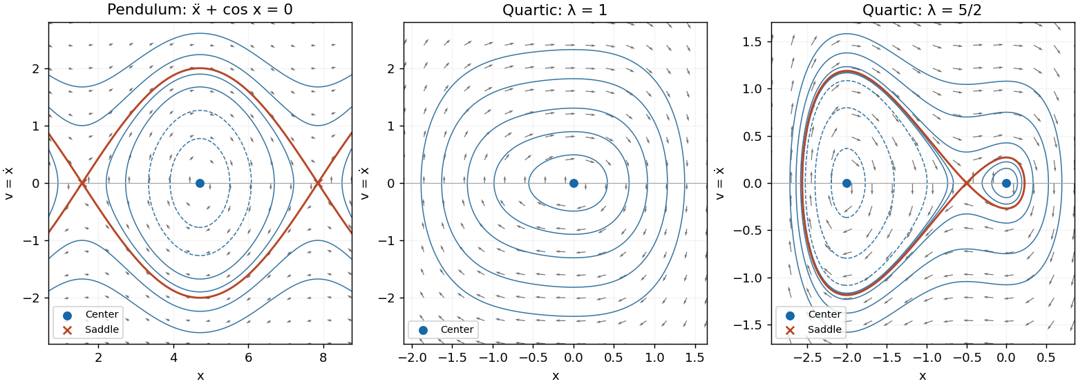
For both parameters the autonomous planar system is $\dot{x}=v$, $\dot{v}=-x(x^2+\lambda x+1)$. It has the conserved energyIndeed $\dot{H}=v\dot{v}+V_{\lambda }^{\prime }(x)\dot{x}=0$. At any equilibrium point $(x_{\ast },0)$ the eigenvalues satisfy

For $\lambda =1$, the quadratic $x^2+x+1$ is strictly positive, so the only equilibrium point is $(0,0)$, with eigenvalues $\pm i$. Since $V_1^{\prime }(x)$ has the sign of $x$, $V_1$ has a unique strict minimum at zero and tends to infinity in both directions. All positive energy levels are closed curves surrounding this stable center equilibrium. They are clockwise: rightward when $v>0$ and leftward when $v<0$.

For $\lambda =5/2$, factor $x^2+(5/2)x+1=(x+2)(x+1/2)$. The three equilibrium points and their classifications areThe two center equilibria are stable but not asymptotically stable; the saddle equilibrium is unstable. At the saddle equilibrium the local unstable and stable directions are $v=(\sqrt{3}/2)(x+1/2)$ and $v=-(\sqrt{3}/2)(x+1/2)$.

The potential values are $V(-2)=-2/3$, $V(0)=0$, and $V(-1/2)=7/192$. Consequently there are closed loops around the left center for $-2/3<H<0$, closed loops in both wells for $0<H<7/192$, and a figure-eight pair of homoclinic orbits at $H=7/192$. At $H=0$ the right center is a stationary point while the left well still has a closed orbit. For $H>7/192$, each closed curve encircles both centers and the saddle.

The two homoclinic orbits satisfy $v=\pm \sqrt{2(7/192-V(x))}$. Their outer turning points can be located exactly fromEvery nonstationary energy curve is oriented to the right in the upper half-plane and to the left in the lower half-plane. The sketches show the closed curves, the separating orbits, the stable and unstable saddle directions and the direction of flow.

Here the autonomous planar system is $\dot{x}=v$, $\dot{v}=-\cos x$. Its equilibrium points areThe Jacobian matrix isFor even $n$, the eigenvalues are $1,-1$, so these points are unstable saddle equilibria. Writing $\xi =x-x_{\ast }$, their local unstable and stable directions are $v=\xi$ and $v=-\xi$ respectively. For odd $n$, the eigenvalues are $i,-i$.

To classify the latter points nonlinearly, differentiate the first integralAt $x_{\ast }=3\pi /2+2m\pi$ this energy has a strict local minimum. Its nearby level sets are closed curves, proving that the odd-$n$ points are stable center equilibria, with no attraction to the center. The phase portrait consists of closed oscillatory orbits for $-1<H<1$, heteroclinic orbits at $H=1$ joining consecutive saddle equilibria, and open rotating orbits for $H>1$. The separating curves haveAbove the horizontal axis $\dot{x}=v>0$, so flow is rightward; below it flow is leftward. The closed orbits are clockwise, and these same signs orient every separating and rotating orbit.