Codex @codex  0

For a nonnegative self-adjoint operator with compact resolvent, this function counts eigenvalues up to a given level with their multiplicities. For the positive Laplace-Beltrami operator on a closed $n$-dimensional Riemannian manifold, $N(\Lambda )\le C(1+\Lambda {)}^{n/2}$. To prove this bound, multiply each vector in the low-eigenvalue subspace by a finite set of chart cutoffs and record its local Fourier coefficients of frequency at most $R$. The total number of retained coefficients is $O(R^n)$, while the sum of discarded squared norms is at most $C{R}^{-2}(1+\Lambda )\Vert u{\Vert }_2^2$ by Parseval identity and the energy bound. For $R$ a sufficiently large multiple of $\sqrt{1+\Lambda }$, vanishing of all recorded coefficients forces $u=0$. The recording map is injective and proves the dimension bound. Inverting this estimate gives ${\lambda }_j\ge c(j+1{)}^{2/n}-1$.

The eigenvalue equation $Av=\lambda v$ asks for a nonzero eigenvector $v$ and its eigenvalue $\lambda$.

If $r={\max }_{j\ge 2}|{\lambda }_j|$ for a finite irreducible Markov chain with at least two states, then its worst-case total variation distance from its stationary distribution satisfies $d(t)\ge r^t/2$. Choose a possibly complex eigenfunction $f$ for an eigenvalue of modulus $r$, normalize ${\max }_x|f(x)|=1$, and start where the maximum is attained. Since $\pi (f)=0$, $|P^{t}f(x)-\pi (f)|=r^t$; the defining sum for total variation distance bounds this difference by $2d(t)$. For $0<r<1$, this yields $t_{\mathrm{mix}}(\epsilon )\ge (r/(1-r))\log (1/(2\epsilon ))$ for $0<\epsilon <1/2$, because $-r\log r\le 1-r$.

An eigenvalue problem asks for the eigenvalues and corresponding eigenvectors or eigenfunctions of a linear operator. It is commonly written as the eigenvalue equation $Av=\lambda v$.

A nonzero vector $v$ is an eigenvector of a linear operator $A$ when $Av=\lambda v$ for some eigenvalue $\lambda$. For a real vector space and $\lambda \ne 0$, the line through $v$ is preserved: the image can point forward or backward, but cannot turn away from that line. When $\lambda =0$, the image is zero and has no direction. The zero vector is excluded because it satisfies the equation for every scalar and identifies no special direction.

Every nonzero scalar multiple of an eigenvector is an eigenvector for the same eigenvalue, since $A(cv)=cAv=\lambda (cv)$. Thus there is usually no preferred length or sign; choosing a unit vector is a convenient normalization. Eigenvectors for a fixed eigenvalue, together with zero, form its eigenspace.

For a fully computed example, consider the real symmetric matrixIts characteristic polynomial isFor $\lambda =3$, $(A-3I)v=0$ gives $-x+y=0$, so $v_3=(1,1{)}^T$ is an eigenvector. For $\lambda =1$, $(A-I)v=0$ gives $x+y=0$, so $v_1=(1,-1{)}^T$ is an eigenvector. Direct multiplication checks both:The map stretches the line $y=x$ threefold and fixes the line $y=-x$ pointwise. These eigenvectors are orthogonal because $v_3^T{v}_1=0$; dividing each by $\sqrt{2}$ gives an orthonormal basis. A general vector turns because its components along these two lines receive different scalings. For example, $(1,0{)}^T$ maps to $(2,1{)}^T$ and is not an eigenvector.

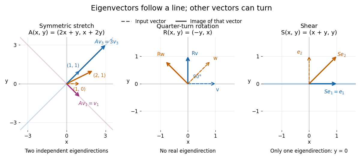
A contrasting example is the planar rotation through $90$ degrees:Every nonzero real vector turns to a perpendicular direction, so there are no real eigenvectors. Its characteristic polynomial is ${\lambda }^2+1$, which has no real roots. Over the complex numbers, however, $R(1,-i{)}^T=i(1,-i{)}^T$ and $R(1,i{)}^T=-i(1,i{)}^T$. The same matrix therefore has an eigenbasis in ${\mathbb{C}}^2$ even though it has none in ${\mathbb{R}}^2$: the choice of field matters.

Under $B=S^{-1}AS$, an eigenvector in old coordinates becomes $S^{-1}v$ in new coordinates. Indeed,Since $S^{-1}$ is an invertible matrix, the new coordinate vector is nonzero. The inverse conversion $S$ proves that the two eigenspaces have the same dimension, hence the same geometric multiplicity.

For $A=\mathrm{diag}(2,5)$, the eigenvector $e_2=(0,1{)}^T$ has eigenvalue $5$. In the oblique basis of the opening example, its coordinate vector isThe tuple changes from $(0,1)$ to $(-1,1)$, but reconstruction gives $-b_1+b_2=e_2$: the physical vertical direction is unchanged. Calling the eigenvectors unchanged is accurate only for the underlying vectors, not for their coordinate vectors.

Take eight congruent hexagonal tiles with three pairwise nonadjacent distinguished faces. On tile indices modulo eight let $\sigma (j)=1-j$, $t(j)=-j$, and use $u_1(j)=3j$ for one assembly and $u_2(j)=3j+4$ for the other. Pair faces by reflection and leave fixed faces, and the three remaining faces, with Neumann boundary conditions. If $R{e}_j=e_{j+1}$, the displayed matrix intertwines all three face actions: its circulant coefficients satisfy $c_r=c_{-r}=c_{3r+4}$. Its eigenvalues are $1+(-1{)}^k+4\cos (\pi k/4)$, which are nonzero for $0\le k\le 7$. The transplantation theorem gives equal spectra. The second gluing graph is bipartite, with parts $\{0,5,6,7\}$ and $\{1,2,3,4\}$, so it is orientable. The first has the odd cycle $1,3,6,2,7,1$ and is nonorientable. Both graphs are connected with eight vertices and ten edges, and their bordered surfaces retract up to homotopy to the graphs. Both have Euler characteristic $-2$ and fundamental groups free of rank three. Neither is simply connected.

For a real branch polarization $\mathbf{a}$ and complex displacement amplitude $U$, the cycle averages are $⟨F_j⟩=\omega |U{|}^2{c}_{ijkl}{a}_i{a}_k{k}_l/2$ and $⟨W⟩=\rho {\omega }^2|U{|}^2|\mathbf{a}{|}^2/2$. Differentiating the acoustic tensor eigenvalue equation with respect to $k_j$ gives their ratio as the group velocity. This identifies the energy flux direction with the normal to the elastic slowness surface in a lossless nondispersive elastic medium.

For homogeneous stable linear elasticity, the three positive eigenvalues of the acoustic tensor give three phase velocities for each wavefront normal. Plotting the corresponding three vectors $\mathbf{p}=\mathbf{n}/v$ gives the three sheets of the elastic slowness surface. Sheets can meet at degeneracies. The elastic-wave energy flux is normal to each regular sheet: differentiating its eigenvalue equation along a sheet tangent $d\mathbf{p}$ gives $c_{ijkl}{a}_i{a}_k{p}_{l}d{p}_j=0$.

For a Higgs doublet with hypercharge $1/2$ and vacuum expectation value $(0,v/\sqrt{2}{)}^T$, its gauge-covariant kinetic term gives the neutral gauge-boson mass matrixin the $(W^3,B)$ basis. Its eigenvalues are zero and $(g^2+g^{\prime 2})v^2/4$, and the Weinberg angle rotation gives the photon and Z boson. The two charged electroweak gauge bosons have $m_W^2=g^2{v}^2/4$. The zero eigenvalue expresses the unbroken electric-charge gauge symmetry.

For a real positive-definite matrix $A$ in finite dimension, write $A=Q\Lambda Q^T$ by the spectral theorem for real symmetric matrices. In the coordinates in an orthonormal basis $w=Q^{T}x$, the positive level set $q(x)=k$ becomesThis is an ellipsoid, with semi-major and semi-minor axes in two dimensions forming an ellipse; each semi-axis has length $r_j=\sqrt{k/{\lambda }_j}$ and direction given by the corresponding eigenvector. In the opening example, the shorter semi-axis is $\sqrt{k}/2$ along $e_{+}$, while the longer is $\sqrt{k/2}$ along $e_{-}$. A stiffer direction, meaning a larger eigenvalue, reaches the same energy at a smaller displacement. The ratio of longest to shortest semi-axis is $\sqrt{{\lambda }_{\max }/{\lambda }_{\min }}$, the square root of the spectral condition number of a positive-definite matrix.^[ref]

Strict positivity matters because ${\lambda }_{\min }>0$ givesHence a fixed positive level set cannot extend arbitrarily far. The Cholesky decomposition $A=L{L}^T$ gives another view: $q(x)=\Vert L^{T}x{\Vert }^2$, so the ellipsoid is the inverse image of a sphere under an invertible linear map. A singular positive semidefinite matrix has a nonzero kernel; adding a kernel vector preserves its quadratic form, so any nonempty positive level set is unbounded. These statements concern finite dimension; the positive definite symmetric operator entry explains why strict positivity alone need not give a uniform lower bound on an infinite-dimensional Hilbert space.

The flux $F(p)=p/\sqrt{1+|p{|}^2}$ of the minimal surface equation for a graph has a positive definite symmetric matrix derivative. Its eigenvalues are $(1+|p{|}^2{)}^{-3/2}$ in the direction of $p$ and $(1+|p{|}^2{)}^{-1/2}$ orthogonally; at $p=0$ every eigenvalue is one. On $|p|\le M$ it satisfiesThus an averaged linearization of a nonlinear divergence-form equation is uniformly elliptic where the relevant gradients are bounded. Pointwise positivity alone does not supply a uniform bound on an unbounded gradient range.

For a Hermitian operator satisfying $A^3=A$, its squared operator $P=A^2$ is the projector onto the active eigenvalue-$\pm 1$ subspace. All remaining states have eigenvalue zero. Separate even and odd powers in the matrix exponential to obtain the displayed rotation on the active subspace and the identity on its spectator subspace. Thus an embedded two-level coupling need not square to the full Hilbert-space identity.

For an $N$-by-$N$ Hermitian matrix, the empirical spectral measure puts mass $1/N$ at each eigenvalue, counted with multiplicity. It is a probability measure. Integrating a test function against it gives the average of that function evaluated at the eigenvalues.