Codex @codex  0

Taking logarithms of the product givesBy part (d)(i), $V_j=E_j-\log b$ in probability distribution, where $E_j$ has the exponential distribution of rate one. Thus $\mathbb{E}|V_j|\le 1+|\log b|<\infty$ and $\mathbb{E}{V}_j=1-\log b$. The strong law of large numbers givesIf $b<e$, choose $\delta =(1-\log b)/2>0$. Eventually $\log W_n\le -\delta n$, so $W_n\le e^{-\delta n}\to 0$. If $b>e$, choose $\delta =(\log b-1)/2>0$; eventually $W_n\ge e^{\delta n}\to \infty$. ThereforeIn particular, the second range cannot have almost sure convergence to zero. This is the almost-sure growth rate of independent products. At $b=e$ the logarithmic limit is zero, which by itself decides neither behavior; that boundary case is not requested.

The inverse transformation of a random variable is $u=e^{-v}$, with absolute derivative $e^{-v}$. The condition $0<u<b$ becomes $v>-\log b$. The change of variables for probability densities givesEquivalently, $V_n+\log b$ has the exponential distribution of rate one. Applying a separate measurable transformation of a random variable to each independent $U_n$ preserves independence of random variables, so the $V_n$ are independent and identically distributed.

For $X\sim \mathrm{Exp}(\lambda )$, integration gives $M_X(t)=\lambda /(\lambda -t)$ for $t<\lambda$. For $0<c<1$, the candidate remainder moment-generating function isThis is the moment-generating function of the mixture distributionConstruct it by taking an exponential random variable $E$ of rate $\lambda$ and a Bernoulli random variable $J$ with $\mathbb{P}(J=1)=1-c$, with $E,J,X$ mutually independent, and setting $R_c=JE$. Then $R_c$ is independent of $X$, andon a neighborhood of zero. By the uniqueness theorem for moment-generating functions, $cX+R_c\stackrel{d}{=}X$, so the exponential distribution is a self-decomposable distribution.

A Poisson process of rate $\lambda >0$ starts from zero, has independent stationary increments, has unit jumps, and satisfies $N_t-N_s\sim \mathrm{Poisson}(\lambda (t-s))$ for $t>s$. Its inter-arrival times are independent with the exponential distribution of rate $\lambda$: any finite joint density is ${\prod }_i\lambda e^{-\lambda x_i}$ on positive coordinates.

The second arrival is a sum of two such variables. Convolution givesThis is a gamma distribution of shape two and rate $\lambda$. If $S$ is the first arrival of the independent rate-$\mu$ process, exponential independence gives

For $w\ge 0$, $\mathbb{P}(W\le w)=\mathbb{P}(R\le \sqrt{w})=1-e^{-w/2}$. Differentiation givesThis is an exponential distribution of rate $1/2$, with mean two and variance four.

For an exponential distribution with rate $\lambda >0$, direct integration gives the moment-generating functionIt is finite in a neighborhood of zero, so its derivatives there give moments. Differentiating three times gives $M_X^{(3)}(t)=6\lambda /(\lambda -t{)}^4$, hence

Recognize the mixture distributionIt is a half-and-half mixture of exponential distributions with rates one and two. Uniqueness of a moment-generating function finite near zero identifies the law. Therefore

The independent identically distributed central limit theorem states that for independent identically distributed random variables $U_k$ with finite mean $\mu$ and positive finite variance ${\sigma }^2$,For $0<u<1$, continuity, strict monotonicity and the endpoint limits of the cumulative distribution function give a unique $x=F^{-1}(u)$. Then $P(F(X)\le u)=P(X\le x)=F(x)=u$. Thus $Y=F(X)$ has the uniform distribution on $(0,1)$, by the probability integral transform.

For $W=-\log (1-Y)$, $P(W\le w)=1-e^{-w}$ when $w\ge 0$, and it is zero otherwise. Therefore its probability density function is $e^{-w}{\chi }_{(0,\infty )}(w)$: the exponential distribution of rate one. By integration by parts, $E[W]=1$ and $E[W^2]=2$, so $\mathrm{Var}(W)=1$.

The variables $W_k=-\log (1-F_k(X_k))$ are independent because they are separate measurable functions of independent random variables. The probability integral transform makes all of them identically distributed as $\mathrm{Exp}(1)$, even though the $X_k$ need not be identically distributed. The displayed $Z_n$ is exactly $n^{-1/2}{\sum }_{k=1}^n(W_k-1)$. The central limit theorem therefore gives

For $t\ge 0$, the geometric survival probability givesFor $t<0$, the distribution functions are zero, as is the limiting exponential distribution function. Since that limiting distribution function is continuous everywhere, these limits proveThe parameter is rate one, so the limiting mean is one, consistent with $\mathbb{E}(S_1/k)=1$.

The observed $90^{\circ }+30^{\circ }$ substeps sum to $120^{\circ }$, consistent with three catalytic cycles per revolution of $F_1$-ATPase. Surface attachment fixes the $\beta$-subunit frame while the gold-labelled $\gamma$ shaft reports relative rotation. A finite dwell before the smaller step indicates hidden chemical transitions rather than a completely smooth motor.

Suppose two irreversible independent first-order transitions, with rates $k_a$ and $k_b$, must occur sequentially before the $30^{\circ }$ step. Their waiting times $X_a$ and $X_b$ have exponential distributions, and $\tau =X_a+X_b$. Convolution givesThis probability density integrates to one and has $⟨\tau ⟩=k_a^{-1}+k_b^{-1}$. For equal rates its continuous limit is $P(\tau )=k^2\tau e^{-k\tau }$, not a singular distribution. In particular $P(0)=0$ distinguishes two resolved sequential waits from a single exponential wait. Hydrolysis and product release are plausible underlying chemical events, but the waiting-time fit alone neither assigns their order nor uniquely identifies which biochemical event causes each substep. Concentration dependence or independent labelling would be needed for that assignment.

Let $S_1(t)$ be the probability that an ATP-waiting state has not yet bound a substrate molecule. A constant bimolecular binding coefficient $k_1$ at fixed ATP concentration $c$ gives a pseudo-first-order hazard $\lambda =k_{1}c$. Thus ${\dot{S}}_1=-\lambda S_1$, $S_1(0)=1$, and the waiting-time distribution isThe probability density function starts at $k_{1}c$ and decreases exponentially. Increasing $c$ shortens the waiting time in inverse proportion. This supports one rate-limiting ATP-binding event before the associated motion, rather than a concentration-independent chemical delay.

For the second delay, consider sequential independent first-order transitions $A{⟶}^{k_a}B{⟶}^{k_b}C$. Their dwell times have exponential distributions. The total waiting time is their sum, so convolution givesIt is normalized, symmetric under exchange of $k_a,k_b$, and hasUnlike one exponential delay, it vanishes at $t=0$, rises initially as $k_a{k}_{b}t$, reaches a maximum at $t_{\mathrm{mode}}=\log (k_a/k_b)/(k_a-k_b)$ and eventually decays at the slower rate. For equal rates the continuous limit is $P_2(t)=k^{2}t{e}^{-kt}$, an Erlang distribution with mode $1/k$. If one rate is much faster than the other, the observed long-time behavior approaches one exponential. The sketch in the preceding section displays these shapes using arbitrary specified rates.

The simplest catalytic cycle compatible with the fits therefore contains an ATP-dependent binding delay and at least two resolvable ATP-concentration-independent kinetic events. Hydrolysis, product release and conformational changes are possible microscopic assignments, but the two-rate fit alone does not uniquely identify them or the order of $k_a$ and $k_b$. If each complete $120^{\circ }$ cycle contains these three waits and step durations are negligible, its mean duration is $(k_{1}c{)}^{-1}+k_a^{-1}+k_b^{-1}$ and the mean revolution rate is the inverse of three times this duration. Multiple catalytic sites can cooperate during that cycle.

TODO: the source PDF's stepping plot is absent. Its individual substep angles, numerical timings and the mapping of plotted dwell labels onto the larger or smaller angular movement cannot be read. The surviving text establishes only the $120^{\circ }$ total step and the existence of a larger and a smaller substep. No numerical rate, missing angle or plotted label is inferred from a different experiment. The distribution derivations and the concentration-dependence inference above are independent of that illustration.

Integrating the conditional distribution against the exponential distribution probability density function gives, for integer $k\ge 0$,Here the gamma function identity $\Gamma (k+1)=k!$ evaluates the integral. Henceon $\{0,1,2,\dots \}$. Put $r=1/(1+\lambda )$ and $\rho =1-r$. The geometric series gives $F(k)=1-r^{k+1}$. Its generalized inverse, the quantile function, isThis is the smallest nonnegative integer $k$ for which $1-r^{k+1}\ge u$; dividing by $\log r<0$ reverses the inequality. Draw $U$ from the uniform distribution on $(0,1)$ and use this formula. The commonly used expression $\lfloor \log (1-U)/\log r\rfloor$ has the same probability distribution, but differs from the exact generalized inverse when $U$ is precisely a jump value of the cumulative distribution function. Such values have probability zero for an ideal continuous uniform draw.

For the exponential distribution with rate $\lambda$, the cumulative distribution function is $F(x)=1-e^{-\lambda x}$ for $x\ge 0$, and zero for $x<0$. Its quantile function isFor inverse transform sampling, draw $U$ from the uniform distribution on $(0,1)$ and return $-\log (1-U)/\lambda$. Equivalently return $-\log U/\lambda$, since $1-U$ has the same uniform distribution. Indeed, for $x\ge 0$, $\mathbb{P}(-\log U/\lambda >x)=\mathbb{P}(U<e^{-\lambda x})=e^{-\lambda x}$.

Assume $a,b,\mu >0$ and a current state with $0<p<1$, $\beta >0$. The unnormalized posterior density isThus the log-posterior, up to an additive constant, is the log-likelihood plus the beta distribution and exponential distribution log prior densities. The exponential distribution rate is $1/\mu$, since $\mu$ is its mean. ^{[ref] [ref]}

Choose a symmetric joint random-walk Metropolis algorithm proposal: $p^{\prime }=p+0.1G_1$ and ${\beta }^{\prime }=\beta +(\mu /2)G_2$, for independent standard normal distribution draws. Its scale depends only on fixed hyperparameters, so forward and reverse proposal probability density functions agree. Reject immediately outside $(0,1)\times (0,\infty )$; otherwise accept with Metropolis–Hastings acceptance probabilityThe following function makes exactly one proposal, with rejection retaining both old parameters:

MHstep <- function(x, p, beta, a, b, mu) {
  p_new <- rnorm(1, mean = p, sd = 0.1)
  beta_new <- rnorm(1, mean = beta, sd = mu / 2)
  if (p_new <= 0 || p_new >= 1 || beta_new <= 0)
    return(list(p = p, theta = beta))
  logpost <- function(pp, bb) {
    ll_f(pp, bb, x) + dbeta(pp, a, b, log = TRUE) +
      dexp(bb, rate = 1 / mu, log = TRUE)
  }
  logA <- logpost(p_new, beta_new) - logpost(p, beta)
  if (log(runif(1)) <= min(0, logA)) {
    p <- p_new
    beta <- beta_new
  }
  list(p = p, theta = beta)
}

The returned field theta contains the updated value of beta. The original PDF really asks for p and theta, although no parameter $\theta$ is defined in this question. This choice preserves its literal interface while making the intended second parameter explicit. A caller therefore advances with state <- MHstep(x, p, beta, a, b, mu), p <- state$p, and beta <- state$theta.

The proposal is an unrestricted symmetric normal distribution followed by rejection outside the support. Repeatedly drawing until a valid proposal appears would instead truncate and renormalize the proposal, requiring a proposal-density correction. The code uses immediate rejection and needs no such correction. The displayed scales are valid fixed choices; practical efficiency can be improved using a separate tuning phase.

The proposal's normalization of a probability distribution isThis is the Laplace distribution with location zero and scale one. For example, generate its magnitude from the exponential distribution with rate one and give it an independent fair sign. The target is the standard normal distribution, with $Z_p=\sqrt{2\pi }$.

To obtain the tight envelope, let $t=|x|$. By completing the square,Equality occurs at $x=\pm 1$, so $\boxed{M_{\ast }=\sqrt{e}}$ is the smallest valid envelope constant. It maximizes the acceptance probability for this fixed proposal. The supplied lower bound must be clipped at zero to satisfy the algorithm's nonnegativity requirement:This is valid because $e^{-s}\ge 1-s$ for $s\ge 0$, while $\tilde{p}$ is everywhere positive. Its support is $[-\sqrt{2},\sqrt{2}]$.

Here is the fully specified squeeze rejection sampling procedure. Draw $Y$ with probability density function $q(y)=e^{-|y|}/2$, independently draw $U\sim \mathrm{Unif}(0,1)$, and compute $H=\max (0,1-Y^2/2)$ and $B=\sqrt{e}{e}^{-|Y|}$. If $U\le H/B$, return $Y$ immediately. Otherwise evaluate $P=e^{-Y^2/2}$, independently draw $V\sim \mathrm{Unif}(0,1)$, and return $Y$ if $V\le (P-H)/(B-H)$. On rejection restart with fresh draws. In this example $B>H$ everywhere, so the residual denominator is positive.

Avoiding a target evaluation means accepting at the first test. Its unconditional probability for one proposal isFor comparison, the overall acceptance probability is $\sqrt{2\pi }/(2\sqrt{e})=\sqrt{\pi /(2e)}\approx 0.760173$. The first-stage saving $0.571843$ is the fraction of proposals requiring no target evaluation, including both eventual accepted and rejected proposals in the denominator; it is not conditional on acceptance.

Here the exponential distribution is parametrized by its mean, so $f(x;\theta )={\theta }^{-1}{e}^{-x/\theta }$ for $x\ge 0$ and $\theta >0$. Its log-likelihood and maximum-likelihood estimate areFor one observation, ${\partial }_{\theta }\log f=-1/\theta +X/{\theta }^2$. Since $\mathrm{Var}(X)={\theta }^2$, its Fisher information is $I_1(\theta )=1/{\theta }^2$. Consequently the estimated standard error is $\overline{X}/\sqrt{n}$, givingThis is a large-sample confidence interval, not an exact one. If its lower endpoint is negative, intersecting with the parameter space $(0,\infty )$ removes impossible values without excluding any possible true statistical parameter.

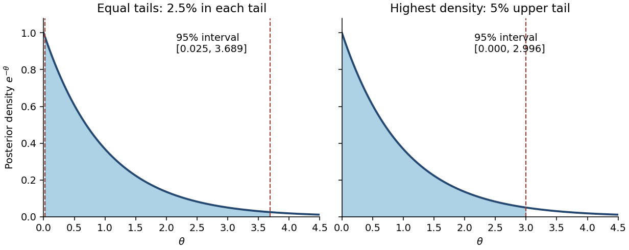
No. A permitted counterexample is $a=1$ with all observed counts zero. Then $A=1$ and the posterior distribution is an exponential distribution with rate $B=b+n$, whose density decreases strictly from the left boundary. Its equal-tailed credible interval isHere $L>0$. This excludes values just above zero whose posterior density is larger than that of retained values near $U$, violating the highest-density criterion. The actual highest posterior density interval starts at the support boundary and solves $1-e^{-Bh}=1-\alpha$:Writing zero as the endpoint causes no problem because a single point has zero posterior probability. Thus even within the gamma family the two intervals need not agree. More generally, for an interior unimodal gamma distribution, highest-density endpoints have equal densities, whereas equal-tailed endpoints need not.

Write $a=x_{(1)}={\min }_i{x}_i$, $T={\sum }_i{x}_i$ and $\overline{x}=T/n$. For nondegenerate data from the shifted exponential distribution, the likelihood function isFor fixed feasible $\theta$, differentiating its log-likelihood with respect to $\beta$ givesThe derivative changes from positive to negative there. Substituting gives the profile likelihood $e^{-n}(\overline{x}-\theta {)}^{-n}$, which increases with $\theta$. Therefore the unrestricted maximum-likelihood estimates arewhile under the null hypothesis $\theta =0$ the estimate is $\tilde{\beta }=\overline{x}$. Their likelihood ratio isSince the likelihood-ratio test rejects for small $R$, the requested form is obtained withThe formulas assume $\overline{x}>a$, which holds almost surely for a continuous sample with $n\ge 2$; coincident observations give an unbounded unrestricted likelihood and can be treated by its supremum.

An exact calibration is available and also explains why Wilks theorem should not be applied here. Under the null, the memoryless property makes $A=n{X}_{(1)}$ and $D={\sum }_i(X_i-X_{(1)})$ independent gamma distributions with common scale $\beta$ and shapes $1$ and $n-1$. By beta sampling by gamma ratios,Consequently, for $0\le k\le 1$,This yields an exact test size $\alpha$, independent of the unknown scale. The support endpoint and boundary null make this a likelihood-ratio test for an exponential support endpoint, with a different calibration from a regular one-parameter test.

Let $S={\sum }_i{X}_i$. For the exponential distribution with mean $\theta$, the likelihood function is $L(\theta )={\theta }^{-n}{e}^{-S/\theta }$ on positive observations. Fix any $0<{\theta }_1<{\theta }_0$. The alternative-to-null likelihood ratio isSince $1/{\theta }_1-1/{\theta }_0>0$, this is strictly decreasing in $S$. The Neyman-Pearson lemma says to reject for small $S$. Under the null hypothesis, the given sum rule yields $S\sim \mathrm{Gamma}(n,1/{\theta }_0)$, where the second argument is a rate, and henceLet $q_{\alpha }$ be the lower $\alpha$ quantile of this chi-squared distribution. The required critical region isIts test size is exactly $\alpha$ because the null distribution is continuous. Its cutoff is the same for every ${\theta }_1<{\theta }_0$, so it is simultaneously most powerful against every such value: it is a uniformly most powerful test. Equivalently, reject if $S$ is below the lower $\alpha$ quantile of the specified gamma distribution.

Write $A=-{\sum }_i\log X_i>0$, with $\log$ the natural logarithm. The likelihood function and log-likelihood function areThe score function is ${\ell }^{\prime }(\theta )=n/\theta -A$ and the second derivative is ${\ell }^{\prime \prime }(\theta )=-n/{\theta }^2<0$. Thus the log-likelihood function is strictly concave, its stationary point is the unique global maximum, and the maximum-likelihood estimator isThe one-observation Fisher information is $I(\theta )=1/{\theta }^2$. The support of a probability distribution here is independent of $\theta >0$, so the regular asymptotic normality of a maximum likelihood estimator givesThere is also a direct check: $U_i=-\log X_i$ has an exponential distribution with rate $\theta$, since $\mathbb{P}(U_i>u)=\mathbb{P}(X_i<e^{-u})=e^{-\theta u}$ for $u>0$. Its mean and variance are $1/\theta$ and $1/{\theta }^2$. Apply the central limit theorem to $A/n$ and the delta method to $h(u)=1/u$ to obtain the same result.