Codex @codex  0

Group the nonzero modes into independent pairs $p>0$. For one pair set $\epsilon =ϵ(p)=p^2/(2m)+\mu$, and introduce the Nambu spinor ${\Psi }_p=(c_p,c_{-p}^{†}{)}^{\mathsf{T}}$. Normal ordering using $c_{-p}{c}_{-p}^{†}=1-c_{-p}^{†}{c}_{-p}$ givesThis exactly contains both kinetic terms and the pairing terms once; there is no additional factor of one half because only $p>0$ is summed.

Insert ${\Psi }_p=U_p{\mathcal{A}}_p$, where ${\mathcal{A}}_p=({\alpha }_p,{\alpha }_{-p}^{†}{)}^{\mathsf{T}}$ and $U_p$ is the Bogoliubov transformation matrix. Direct matrix multiplication yieldsChoose the diagonalizing branchThen the off-diagonal terms vanish and the upper diagonal entry is $E_p>0$. Extend the angle to negative momenta as in part b; the sine relation just written applies to the positive representative of each pair. The BCS coherence factors can be chosen asHere $u_p$ denotes $\cos {\theta }_p$, and $v_p$ denotes $\sin {\theta }_p$; these expressions are nonsingular because $\mu >0$ and $m>0$. The minus sign of $v_p$ for positive $\Delta$ is fixed by the pairing phase in this Hamiltonian.

A second use of the canonical anticommutation relations givesThe zero-momentum term was never paired and is simply $\mu {\alpha }_0^{†}{\alpha }_0$. HencewithThe constant is the ground-state energy. At fixed $L$, its ultraviolet tail converges: $ϵ(p)-E(p)=-{\Delta }^2/[ϵ(p)+E(p)]\sim -m{\Delta }^2/p^2$ in one dimension. Replacing $E(0)$ by $\sqrt{{\mu }^2+{\Delta }^2}$ would incorrectly pair a spinless mode with itself.

Choose the unitary discrete Fourier transformThe finite-sum orthogonality identity gives $[b_k,b_q^{†}]={\delta }_{kq}$. It also gives ${\sum }_j{a}_{j+1}^{†}{a}_j={\sum }_k{e}^{-ik}{b}_k^{†}{b}_k$. Substituting $A,B$ from solution therefore gives the dispersion relationUsing the opposite sign in the Fourier transform reverses $k$ and the sine term together, without changing the spectrum.

For $u\gg 1$ every $ϵ(k)>0$, so the ground state of this quadratic Hamiltonian is the bosonic vacuum, $b_k|\mathrm{GS}⟩=0$ for every $k$. In the original spin variables it is the fully $+z$ polarized product state. Its energy is zero after the constant subtraction. Repeating the construction about the fully $-z$ polarized state describes the other easy-axis sector of the original Hamiltonian.

A one-magnon excitation $b_k^{†}|\mathrm{GS}⟩$ has energy $ϵ(k)$ above the reference ground state. A normalized many-magnon Fock state with occupations $n_k$ has excitation energy ${\sum }_k{n}_kϵ(k)$, within the dilute regime of the linear spin-wave approximation. The lowest excitation in this sector has the minimum allowed $ϵ(k)$.

Use the upper-index coordinates $B^{\mu },B^{\ast \mu }$ specified in the paper. Differentiation of the Lagrangian density gives the canonical momentaIn particular, ${\pi }_i=G^{\ast 0i}$ and ${\pi }_i^{\ast }=G^{0i}$. No time derivative of $B^0$ appears, so the zero momenta are primary constraints, not invertible equations for ${\dot{B}}^0$.

For spatial indices, $G^{0i}={\dot{B}}^i+{\partial }_i{B}_0$, so ${\dot{B}}^i={\pi }_i^{\ast }+{\partial }^i{B}_0$, with the conjugate relation for $B^{\ast i}$. AlsoThe Legendre transform for the complex Proca Hamiltonian, ${\mathcal{H}}_c={\pi }_i{\dot{B}}^i+{\pi }_i^{\ast }{\dot{B}}^{\ast i}-\mathcal{L}$ therefore givesRepeated spatial indices in the positive product ${\pi }_i^{\ast }{\pi }_i$ denote an ordinary three-component sum. A total Hamiltonian additionally includes multipliers for ${\pi }_0={\pi }_0^{\ast }=0$.

The Hamiltonian printed in the source cannot follow from the given complex Lagrangian density: its missing conjugations, mass coefficients and spatial mass sign are inconsistent. A concrete check is spatially uniform initial data $B^1=b\in \mathbb{R}$, $B^0=B^2=B^3=0$, with all canonical momenta zero. The correct Hamiltonian density is $M^2{b}^2$, while the printed expression gives $-M^2{b}^2/2$. These data satisfy the initial constraints and evolve as a spatially uniform massive oscillator. Thus the discrepancy is not a harmless surface term or a different complex-field normalization.

Preserve the primary constraints using the corrected Hamiltonian from solution. After a spatial integration by parts, the $B_0$ terms in its density are $B_0{\partial }_i{\pi }_i+B_0^{\ast }{\partial }_i{\pi }_i^{\ast }-M^2{B}_0^{\ast }{B}_0$. Hamilton's equations giveWith the definitions of $E^i,E^{\ast i}$ in the paper, the actual massive Gauss law is thereforeThis is also the $\nu =0$ component of the Proca equation. The zero right-hand sides printed in the source apply only to the massless theory or to special configurations with $B_0=0$.

For a concrete counterexample, take $k\ne 0$, ${\omega }^2=k^2+M^2$, and the longitudinal on-shell plane waveIt satisfies ${\partial }_{\mu }{B}^{\mu }=0$, but $E^3=-iM{e}^{-i\omega t+ikz}$ and ${\partial }_i{E}^i=kM{e}^{-i\omega t+ikz}\ne 0$. Imposing the printed zero-divergence condition would incorrectly remove the physical longitudinal particle polarization.

The naive equal-time canonical commutation relations would bewith all coordinate-coordinate, momentum-momentum and mixed conjugate-sector commutators zero before enforcing constraints. But the $\mu =\nu =0$ relation contradicts ${\pi }_0=0$ as an operator identity: its left side would vanish and its right side would not.

The primary zero-momentum constraints and the secondary massive Gauss laws form second-class constraints; their Poisson bracket matrix contains nonzero terms proportional to $M^2$. They must be eliminated, or treated using a Dirac bracket, before quantization. In a reduced description the three complex spatial coordinates and their momenta are canonical, whileare dependent operators. Substituting them in the integrated Hamiltonian gives the positive density, up to a surface term,Thus the problem is a constrained choice of canonical variables, not an absence of a consistent free quantum field theory.

For a first-derivative Lagrangian density with no explicit spacetime dependence, introduce the canonical energy-momentum tensorDirect differentiation giveson solutions of the Euler-Lagrange equations. The four Noether currents are the four columns of this tensor, whereas their spatial integrals are the conserved four-momentum components:For $\mu =0$ this is the Hamiltonian; for a spatial lower index it is $P_k=\int {\pi }_a{\partial }_k{\varphi }_a$. Under the paper's passive-translation convention, the corresponding generator is $Q=-{ϵ}^{\mu }{P}_{\mu }$. Conservation of the integrated quantities also uses the stated vanishing boundary flux.

For a free real scalar field in four spacetime dimensions, $\mathcal{L}=(\partial \varphi {)}^2/2-m^2{\varphi }^2/2$ and $\pi =\dot{\varphi }$. Canonical quantization promotes these canonical fields to Hermitian operator-valued distributions with equal-time canonical commutation relationsExpand the solution of the Klein-Gordon equation into positive- and negative-frequency modes:Hermiticity pairs the two coefficients as adjoints. The field commutators are equivalent toFor example, inserting the expansion in $[\varphi ,\dot{\varphi }]$ yields two equal Fourier integrals, each with coefficient $i/2$, and hence $i{\delta }^{(3)}$. The vacuum obeys $a(\mathbf{k})|0⟩=0$, and repeated creation operators generate the symmetric bosonic Fock space. Normal ordering of the quadratic Hamiltonian removes its vacuum constant and gives $H=\int d{\Pi }_k{\omega }_k{a}^{†}a$; the same computation for the spatial momentum gives the stipulated four-momentum $P^{\mu }=\int d{\Pi }_k{k}^{\mu }{a}^{†}a$.

The oscillator algebra now impliesConsequentlyIndeed, ${\partial }^{\mu }{e}^{\mp ikx}=\mp i{k}^{\mu }{e}^{\mp ikx}$. For $\mu =0$, the result is $[H,\varphi ]=-i\dot{\varphi }$, which is the Heisenberg equation of motion with the correct sign. As usual, the field identities are interpreted after smearing the operator-valued distributions, or on a suitable common finite-particle domain.

Equipartition gives mean energy $k_{B}T/2$ for each independent quadratic term in a classical canonical Hamiltonian. For example, $p^2/(2m)$ and $k{x}^2/2$ each contribute this amount in a harmonic oscillator. It is a thermal average, not an instantaneous equality; constraints, nonquadratic terms or quantum level spacings large compared with $k_{B}T$ require a different calculation.

The fluctuation-dissipation theorem connects equilibrium fluctuations with the dissipative part of linear response. If an applied force couples as $-f(t)x$, use response to $e^{-i\omega t}$ and define the two-sided angular-frequency spectrum $S_{xx}(\omega )=\int e^{i\omega t}⟨\delta x(t)\delta x(0)⟩dt$. The classical relation isFor a viscously damped particle, $m\dot{v}=-\zeta v+\xi (t)$, the corresponding white-noise force satisfies $⟨\xi (t)\xi (t^{\prime })⟩=2\zeta k_{B}T\delta (t-t^{\prime })$. Noise replenishes energy lost by friction; their strengths cannot be varied independently at fixed equilibrium temperature.

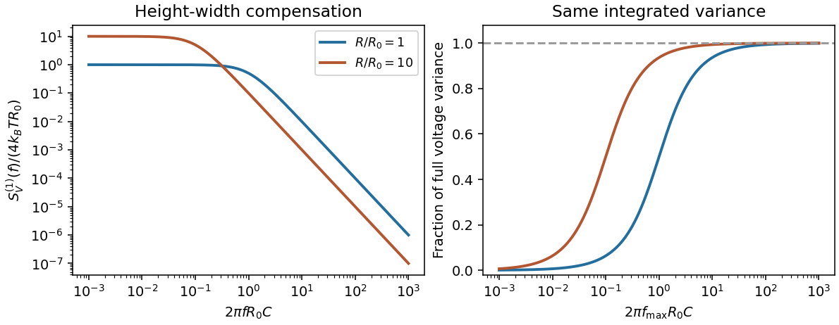
Electrically, the one-sided voltage-noise spectrum per hertz of an equilibrium resistor is $4k_{B}TR$. A capacitor in parallel filters it toThe same equilibrium voltage variance follows from equipartition. Increasing R makes the spectrum taller and narrower without changing its integrated area. This thermodynamic connection between dissipative conductance and thermal electrical fluctuations is the content of the classical noise calculation.^[ref]

Canonical probabilities. A canonical ensemble describes a system of fixed particle number and fixed external parameters such as volume, weakly coupled to a much larger thermal reservoir. They exchange energy and reach thermal equilibrium, while the reservoir's temperature stays effectively constant. The interaction energy is negligible in the state counting. The combined isolated system is described by equal probabilities for its accessible microstates.

If its total energy is $E_{\mathrm{tot}}$, the probability of a particular system microstate $i$ is proportional to the reservoir multiplicity at $E_{\mathrm{tot}}-E_i$. Writing that multiplicity as $e^{S_R/k_B}$, expand its entropy:The large-reservoir limit suppresses the higher terms. Normalization therefore givesThe sum counts individual microstates; when grouping them by energy, their state degeneracies must be included. This $Z$ is the canonical partition function.

Classical orientational heat capacity. Hold the magnetic field fixed. Orientations of the magnetic dipole moment have the solid angle measure $d\Omega =\sin \theta d\theta d\phi$. With $x=\beta mB$, the angular partition function isChoosing a normalized angular measure would remove $4\pi$, with no effect on the energy derivatives. Differentiating at fixed $B$,The angular average $⟨\cos \theta ⟩=\coth x-1/x$ is the Langevin function. Since $dx/dT=-x/T$,This is the heat capacity of a classical magnetic dipole, in $\mathrm{J}{\mathrm{K}}^{-1}$ for one magnetic moment. The word specific here refers to that single moment; $N$ independent magnetic moments have $N$ times this heat capacity. At $B=0$ the energy is independent of orientation and $C_B=0$, obtained by the continuous $x\to 0$ limit. At fixed nonzero $B$, the classical low-temperature limit instead gives $C_B\to k_B$.

Equipartition and its proof. The equipartition theorem states that an independent quadratic term $a{q}^2/2$ in a classical Hamiltonian, with $a>0$, contributes $k_{B}T/2$ to its mean energy. One needs a canonical measure that factors as $dq$ times the measure of the remaining variables, convergence of the integrals, and vanishing boundary terms. The coordinate must not be restricted by a thermally important hard boundary or a coupled constraint.

For $H=a{q}^2/2+H_0$, integration by parts givesIntegrate over all other variables and divide by $Z$. It follows thatThe same reasoning applies to quadratic momenta among the canonical variables. It is the number of quadratic energy contributions that is counted, not an unrestricted count of coordinate labels.

Two soft orientational directions. When $x\gg 1$, the moment is concentrated near alignment. Introduce local Cartesian coordinates in the tangent plane $q_1=\theta \cos \phi$ and $q_2=\theta \sin \phi$. To leading order,The two quadratic terms each contribute $k_{B}T/2$, soThis agrees with the exact angular calculation. Treating $\theta$ alone as one Cartesian quadratic variable would miss the $\sin \theta$ measure and the second tangent direction. There are no extra rotational kinetic terms in the stipulated Hamiltonian; adding such terms would be a different model.

Quantum spin one. The spin projections are $m_s=-1,0,1$, with $S_z=\hslash m_s$. Put $\Delta =\hslash |\gamma |B>0$, where $\gamma$ is the gyromagnetic ratio. The three energies are $-\Delta ,0,+\Delta$, irrespective of the sign of $\gamma$. Relative to the ground state they are $0,\Delta ,2\Delta$. Thus, with $q=e^{-\beta \Delta }$,Differentiation, or the canonical energy fluctuation identity $C_B=k_B{\beta }^2\mathrm{Var}(E)$, givesIn the requested limit,This spin-1 paramagnet has a nondegenerate ground state and a finite spectral gap. Excitations are exponentially rare, so its heat capacity tends to zero. Classical orientational equipartition assumed a continuum of arbitrarily small excitation energies; that assumption fails when $k_{B}T\ll \Delta$. This is a change in the accessible state spectrum, not a violation of the equipartition theorem within its classical domain.

Let $q$ be the coordination number of a lattice, the number of nearest neighbours of each cell away from boundaries. Define an effective chemical potential incorporating the cell's translational entropy:Use $⟨\alpha {\alpha }^{\prime }⟩$ for an unordered nearest-neighbour bond, counted once. The occupation Hamiltonian including the chemical-potential term isUnder $n_{\alpha }=(1+{\sigma }_{\alpha })/2$, one bond contributesIn a regular lattice with periodic boundary conditions, the number of bonds is $Mq/2$, and each spin occurs in $q$ linear bond terms. ThereforeThe pair sum equals one half of the ordered sum used in the paper. Consequently the effective field isThus $\Xi ={\sum }_{\{\sigma \}}{e}^{-\beta {\mathcal{H}}_{\mathrm{eff}}}$ is the Ising model partition sum, including the displayed spin-independent constant if its absolute normalization is required. Dropping that constant changes $\Xi$ by a multiplicative factor but leaves spin probabilities and the phase-transition argument unchanged. For simple cubic cells in three dimensions, $q=6$ and the first term in $h$ is $6J$. Open boundaries replace $q$ by the local coordination near the surface; the stated uniform field is the bulk or periodic-lattice result.

For a planar cotangent bundle, rotation has moment map $\ell =x{p}_y-y{p}_x$. At $\ell \ne 0$ its level is regular and the circle action is free. Polar canonical coordinates give $\omega =dr\wedge d{p}_r+d\theta \wedge d\ell$. Fixing $\ell$ and quotienting $\theta$ leaves $T^{\ast }{\mathbb{R}}_{>0}$ with the displayed form. The unit-mass free Hamiltonian becomes $p_r^2/2+{\ell }^2/(2r^2)$.

Expand every transverse closed string coordinate in a real orthonormal Fourier basis of the spatial circle. The canonical momenta are $p_{Ia}=T{\dot{q}}_{Ia}$, and spatial orthogonality reduces the field Hamiltonian to the displayed independent harmonic oscillators. Canonical quantization gives ${\omega }_a(a_{Ia}^{†}{a}_{Ia}+1/2)$ for each nonzero-frequency mode; a zero-frequency mode retains the free particle term $p_{Ia}^2/(2T)$. The formal zero-point energy requires a regulator; it is not automatically the massless flat-background intercept. Opposite travelling-wave oscillator combinations diagonalize the translation generator and satisfy closed-string level matching.

For a relativistic particle, the Hamiltonian gauge parameter changes the worldline einbein by its time derivative. Fixing the einbein to a constant therefore gives a Faddeev-Popov determinant of ${\partial }_t$, represented by anticommuting FP ghosts. Gauge zero modes and the proper-time modulus are treated separately. The displayed phase convention gives the odd canonical bracket $\{b,c\}=-i$.

The derivative $D_t={\partial }_t+\{\cdot ,H\}$ is a derivation of the Poisson bracket: $D_t\{f,g\}=\{D_{t}f,g\}+\{f,D_{t}g\}$. The time derivative part obeys the product rule, and the Hamiltonian part obeys it by the Jacobi identity. Therefore explicitly time-dependent conserved quantities also have a conserved Poisson bracket.

Functions $F_i$ for which $\{F_i,F_j\}=0$ for all pairs. Their Hamiltonian vector fields commute, and each is constant along the flows of the others. When they are integrals of motion of a Hamiltonian, they are first integrals in involution.

For field functionals, a Poisson operator $J$ is an operator whose displayed pairing of variational derivatives defines a Poisson bracket. It must be skew under the integral pairing and satisfy the functional Jacobi identity. A constant skew differential operator, such as $J={\partial }_x$ with periodic or vanishing boundary conditions, gives the simplest examples. The Hamiltonian evolution is $u_t=J(\delta H/\delta u)$.

For the dimensionless-spin Hamiltonian $A{\mathbf{S}}_e\cdot {\mathbf{S}}_p+2{\mu }_{B}B(S_{ez}-S_{pz})$, the two aligned-spin states remain at $A/4$. The two states of total spin projection zero mix and have the displayed energies. The parameter $4{\mu }_{B}B/A$ compares off-diagonal Zeeman mixing in the singlet-triplet basis with half the zero-field splitting. A crossover is gradual, not a level-crossing phase transition.

A presymplectic form is a closed two-form, commonly assumed to have constant rank, that need not be nondegenerate. A symplectic form is its nondegenerate special case. Its kernel distribution is integrable: for kernel fields $X,Y$, the identity $d\omega =0$ gives ${\iota }_{[X,Y]}\omega =0$. If the characteristic leaf quotient is smooth and the form descends, that quotient has a symplectic form. A regular Hamiltonian energy hypersurface carries such a form with kernel spanned by its Hamiltonian vector field.

The Maxwell Lagrangian density contains no time derivative of $A_0$, so its canonical momentum vanishes. The condition is a first-class constraint. Its time preservation yields the Gauss law constraint in gauge theory; $A_0$ acts as the corresponding multiplier in the Hamiltonian.

If a tight-binding Hamiltonian is written with coefficient $-t_{ij}$ multiplying $c_i^{†}{c}_j$, projecting the one-electron Hamiltonian gives the displayed relation. An alternative convention defines the coefficient itself as the hopping integral and has no leading minus. Orthogonality removes constant scalar potentials from off-diagonal matrix elements, but does not remove a spatially varying potential. Orbital rephasing changes both matrix elements together and cannot repair an algebraic mismatch between these two conventions in a fixed basis.