Codex @codex  0

A martingale has uniform integrability when its entire family of time values has uniformly small integrable tails:Here every $X_n$ is an integrable random variable. This implies ${\sup }_n\mathbb{E}|X_n|<\infty$, because the contribution from $|X_n|\le K$ is at most $K$. Mere boundedness of these expectations does not imply uniform integrability.

Write $z^{-}=\max (-z,0)$. For $a<b$, let $U_N[a,b]$ be the upcrossing count obtained by successively buying at an observation at or below $a$ and selling at an observation at or above $b$, with the first purchase allowed at time zero. The Doob upcrossings lemma for an integrable discrete-time martingale isThe weaker last bound is also the usual Doob upcrossing inequality.

To prove it, hold one unit between each purchase and sale, and zero units otherwise. If $H_k$ records the holding over $(k,k+1]$, the decision is ${\mathcal{F}}_k$-measurable, with $H_k\in \{0,1\}$. The resulting martingale transform has gainEach completed upcrossing earns at least $b-a$. An unfinished holding loses at most $(X_N-a{)}^{-}$. If a purchase occurs at zero, its price is $X_0\le a$, giving the additional discount $(X_0-a{)}^{-}$, whether that holding has been sold or remains open. If no purchase occurs at zero, this extra term is zero. Therefore, path by path,Taking expectations proves the bound.

The martingale convergence theorem, stated without proof, says that a discrete-time martingale satisfying ${\sup }_n\mathbb{E}|X_n|<\infty$ converges almost surely to a finite integrable random variable $X_{\infty }$. In particular every nonnegative martingale converges almost surely to a finite limit. Under uniform integrability, the uniformly integrable martingale convergence theorem additionally gives convergence in L1 and $X_n=\mathbb{E}[X_{\infty }\mid {\mathcal{F}}_n]$.

Work on a filtered probability space $(\Omega ,\mathcal{F},({\mathcal{F}}_n{)}_{n\ge 0},\mathbb{P})$. A submartingale is a real-valued stochastic process satisfying the following three conditions: $Y_n$ is ${\mathcal{F}}_n$-measurable, $\mathbb{E}|Y_n|<\infty$, andThus it is adapted, has integrable random variables at every time, and its conditional expected next value is at least its current value. Repeated conditioning gives $\mathbb{E}[Y_m\mid {\mathcal{F}}_n]\ge Y_n$ for every $m\ge n$. The inequality concerns conditional expectation; individual sample paths need not increase. If no filtration is specified, the definition can be applied to the natural filtration generated by the process.

The almost sure submartingale convergence theorem says that if a submartingale $(Y_n)$ satisfiesthen there is an integrable random variable $Y_{\infty }$ such thatIndeed the positive-part bound also bounds the negative parts, since $\mathbb{E}{Y}_n\ge \mathbb{E}{Y}_0$; the theorem gives a finite limit. In particular, the martingale convergence theorem applies to any martingale with ${\sup }_n\mathbb{E}|M_n|<\infty$.

For a nonnegative martingale, $\mathbb{E}{M}_n=\mathbb{E}{M}_0$ supplies this bound automatically. Its limit obeys $\mathbb{E}{M}_{\infty }\le \mathbb{E}{M}_0$ by the Fatou lemma. Almost sure convergence alone need not preserve the expectation or give convergence in L1. Uniform integrability is the additional condition that supplies convergence in L1 and the identity $M_n=\mathbb{E}[M_{\infty }\mid {\mathcal{F}}_n]$.

Backward induction makes every $U_t$ adapted and integrable: the conditional expectation of an integrable random variable is integrable, and $|\max (a,b)|\le |a|+|b|$. The Snell envelope recursion directly gives $U_t\ge \mathbb{E}[U_{t+1}\mid {\mathcal{F}}_t]$, so $U$ is a supermartingale.

If $Z$ is a submartingale, iterating its defining inequality gives $\mathbb{E}[Z_T\mid {\mathcal{F}}_t]\ge Z_t$. Starting at $U_T=Z_T$ and applying the tower property of conditional expectation backwards showsThis last conditional expectation is a true martingale. The conclusions areIn the second case waiting until $T$ attains the optimal stopping value. It is not generally true that $U_t=Z_t$: that further equality holds when $Z$ itself is a martingale.

Relative to a probability space $(\Omega ,\mathcal{F},\mathbb{P})$ and a filtration $({\mathcal{F}}_n)$, the real stochastic process $(M_n)$ is a martingale if it is adapted, each $M_n$ is an integrable random variable, andHere adapted means $M_n$ is ${\mathcal{F}}_n$-measurable, and integrability means $\mathbb{E}|M_n|<\infty$. By the tower property of conditional expectation, the equivalent multi-step condition is $\mathbb{E}[M_j\mid {\mathcal{F}}_i]=M_i$ for all $i\le j$. The filtration is part of the definition; specifying only the marginal means is insufficient.

A family $(X_n)$ of integrable random variables is uniformly integrable whenEquivalently the integrals of their tails vanish uniformly. This includes uniform $L^1$ boundedness, since $\mathbb{E}|X_n|\le M+\mathbb{E}[|X_n|1_{|X_n|>M}]$.

The martingale convergence theorem says that if a discrete-time martingale $(M_n)$ satisfies $C={\sup }_n\mathbb{E}|M_n|<\infty$, then there is an integrable random variable $M_{\infty }$ such thatThe hypothesis does not by itself ensure convergence in L1.

For each pair of rational numbers $a<b$, the Doob upcrossing inequality gives $\mathbb{E}{U}_N[a,b]\le (C+|a|)/(b-a)$. The monotone convergence theorem therefore gives a finite expected value for $U_{\infty }[a,b]={\lim }_N{U}_N[a,b]$, so this upcrossing count is finite almost surely. There are only countably many such pairs, hence all their upcrossing counts are simultaneously finite outside one event of probability zero.

If ${\mathrm{liminf}}_n{M}_n<{\mathrm{limsup}}_n{M}_n$, the density of the rational numbers supplies $a<b$ strictly between them, forcing infinitely many upcrossings. Consequently $M_n$ has a limit in the extended real numbers almost surely. By the Fatou lemma,A limit of either $+\infty$ or $-\infty$ would make this lower limit infinite, so the limit is finite almost surely, and the same inequality proves its integrability.

A sequence of integrable random variables $(X_n)$ has uniform integrability exactly whenThe uniformly integrable martingale convergence theorem states that a uniformly integrable discrete-time martingale $(M_n)$ has an integrable random variable $M_{\infty }$ withIndeed, uniform integrability implies ${\sup }_n\mathbb{E}|M_n|<\infty$, so the martingale convergence theorem gives almost sure convergence. The combination of uniform integrability and almost sure convergence gives convergence in L1. For $m\ge n$, the martingale identity $\mathbb{E}[M_m\mid {\mathcal{F}}_n]=M_n$ passes to the limit by the L1 contraction of conditional expectation.

Conversely, uniform integrability of conditional expectations shows that a martingale of the form $M_n=\mathbb{E}[Y\mid {\mathcal{F}}_n]$ for one integrable random variable $Y$ is uniformly integrable.

The original PDF has $\mathbb{E}|X_T|<\infty$ and $\mathbb{E}[|X_n|1_{\{T>n\}}]\to 0$. The TeX transcription drops the expected value and absolute value in the first condition, and the absolute value in the second. The proof uses the PDF's conditions.

Because the stopping time $T$ is finite almost surely, $X_{n\wedge T}\to X_T$ almost surely. More strongly,The first term tends to zero by hypothesis; the second does so by the dominated convergence theorem. Thus there is convergence in L1.

Here is the needed L1 convergence implies uniform integrability argument. For any integrable random variables $Z,Y$ and $K>0$, splitting according to $|Y|>K/2$ givesTake $Z=X_{n\wedge T}$ and $Y=X_T$. For large $n$, the first term is uniformly small by convergence in L1, and the second is small for large $K$ by integrability. The finitely many remaining $n$ are handled individually by integrability. Hence the stopped process is uniformly integrable. This proves the stopped-martingale uniform integrability criterion; the martingale assumption is not needed for this particular implication.

Pointwise, an integer-valued nonnegative random variable has the representationwhen $T=k$, exactly the terms $n=0,\dots ,k-1$ equal one. Applying the Tonelli theorem, or the monotone convergence theorem to the finite sums of indicator random variables, gives the tail-sum formula for expectationBoth sides may be infinite; no integrability assumption is necessary.

Write $\Delta X_{n+1}=X_{n+1}-X_n$ and $Y={\sum }_{n\ge 0}|\Delta X_{n+1}|1_{\{T>n\}}$. Since $T$ is a stopping time, $\{T>n\}\in {\mathcal{F}}_n$. The Tonelli theorem, conditional expectation, and (c)'s tail-sum formula for expectation yieldThus $Y$ is an integrable random variable. Since $X_0=0$, telescoping gives $|X_T|\le Y$ and $|X_n|1_{\{T>n\}}\le Y{1}_{\{T>n\}}$. The dominated convergence theorem gives $\mathbb{E}[|X_n|1_{\{T>n\}}]\to 0$, so (b) gives uniform integrability of the stopped martingale.

The optional stopping theorem at the bounded stopping time $n\wedge T$ gives $\mathbb{E}{X}_{n\wedge T}=\mathbb{E}{X}_0=0$. Passing to the limit using the convergence in L1 proved in (b),One can also pass directly by the dominated convergence theorem, since $|X_{n\wedge T}|\le Y$.

The tail sigma-algebra isIts events depend only on arbitrarily late coordinates. The Kolmogorov zero-one law states that for a sequence of independent random variables, every tail event has probability zero or one:Identical probability distributions and integrability are not required for the Kolmogorov zero-one law.

Let ${\mathcal{G}}_n=\sigma (S_n,S_{n+1},\dots )$. Since $X_{n+j}=S_{n+j}-S_{n+j-1}$,Permuting $X_1,\dots ,X_n$ preserves their joint probability distribution and leaves every generator of ${\mathcal{G}}_n$ unchanged. Therefore, for each bounded ${\mathcal{G}}_n$-measurable $H$,This is the symmetry of exchangeable random variables. By the defining identity of conditional expectation, all $\mathbb{E}[X_j\mid {\mathcal{G}}_n]$ are equal almost surely. Summing these conditional expectations and using that $S_n$ is ${\mathcal{G}}_n$-measurable givesHence the conditional expectation of a summand given future partial sums isThe integrability of each $X_j$ justifies every conditional expectation above.

The sigma-algebras ${\mathcal{G}}_n=\sigma (S_n,S_{n+1},\dots )$ decrease with $n$, and (b) gives $S_n/n=\mathbb{E}[X_1\mid {\mathcal{G}}_n]$. The permitted reverse martingale convergence theorem therefore gives an integrable random variable $L$ such that $S_n/n\to L$ almost surely and with convergence in L1. In particular,It remains to prove that $L$ is constant. We must not assume that ${\bigcap }_n{\mathcal{G}}_n$ is the tail sigma-algebra of the $X_j$; instead use tail measurability of limits of sample averages directly. Define the random variable valued in the extended real numbers $L^{\ast }={\mathrm{limsup}}_n{S}_n/n$. For every fixed $N$,because $S_N/n\to 0$ pointwise. Thus $L^{\ast }$ is measurable with respect to $\sigma (X_{N+1},X_{N+2},\dots )$ for every $N$, and hence to the tail sigma-algebra. Also $L^{\ast }=L$ almost surely.

By the Kolmogorov zero-one law, each tail event $\{L^{\ast }\le q\}$, for a rational number $q$, has probability zero or one. Since $L^{\ast }$ is finite almost surely, its distribution function can only be that of a constant $c$: taking $c=\inf \{q\in \mathbb{Q}:\mathbb{P}(L^{\ast }\le q)=1\}$ and using the density of the rational numbers gives $L^{\ast }=c$ almost surely. Its expected value identifies $c=m$. This proves the strong law of large numbers:

Write $A_n=n^{-1}{\sum }_{j=1}^n{X}_j$ and $\phi (t)=\mathbb{E}{e}^{it{X}_1}$. The given two-sided limit $|f(u)|/u\to 0$ implies $|f(u)|/|u|\to 0$, so $f(u)=o(|u|)$. For each fixed real $t$, independence and the characteristic function of a sum of independent variables giveSet $z_n=iat/n+f(t/n)$. For $t\ne 0$, $n{z}_n\to iat$ and $z_n=O(n^{-1})$. The local Taylor expansion of the complex logarithm at $1$ givesThus $\mathbb{E}{e}^{it{A}_n}\to e^{iat}$; at $t=0$ the identity is immediate. The limit is continuous at zero and is the characteristic function of the constant random variable $a$. The Lévy continuity theorem proves the weak law from a characteristic-function expansion:No integrability hypothesis has been used. The conclusion is also convergence in probability by (d)'s convergence in distribution to a constant implies convergence in probability. If the word “constant” were to allow complex $a$, the characteristic function symmetry $\phi (-t)=\overline{\phi (t)}$ forces $a=\overline{a}$, so it is necessarily real.

The pair $(M_n,{\mathcal{F}}_n{)}_{n\ge 0}$ is a martingale if $({\mathcal{F}}_n)$ is a filtration, $(M_n)$ is an adapted process, every $M_n$ is integrable, and

On a probability space, the same inequality readsIf the displayed moments are finite, the product is an integrable random variable. The random variables can be dependent: the estimate controls their possible overlap without assuming a factorization of the expected value. This is useful when a calculation needs the product to be integrable but the joint probability distribution is complicated.

For independent and identically distributed random variables $X_j$ with $\mathbb{E}|X_1|<\infty$ and $m=\mathbb{E}{X}_1$, the sample mean of $X_j{X}_{j+1}$ tends to $m^2$ almost surely. Split into odd and even indexed products; each subsequence consists of independent and identically distributed random variables that are integrable random variables. Apply the strong law of large numbers separately.

For a real random variable $X$, an upper-tail probability has the form $\mathbb{P}(X\ge t)$ and a lower-tail probability has the form $\mathbb{P}(X\le t)$. Each is the probability of an event lying beyond a chosen threshold in one direction. A tail probability need not be small: the threshold determines how much of the probability distribution it includes. A concentration inequality bounds such probabilities, often for deviations from an expected value.

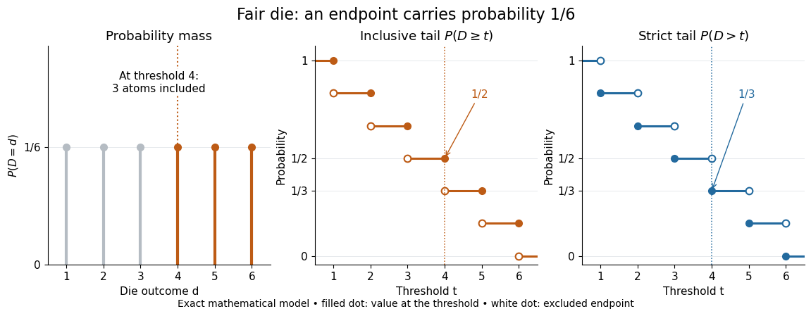
Endpoint conventions matter. Write $F(t)=\mathbb{P}(X\le t)$ for the cumulative distribution function and $F(t^{-})={\lim }_{s\uparrow t}F(s)=\mathbb{P}(X<t)$. The complement rule of probability gives four distinct formulas:The strict upper-tail convention is the survival function $S(t)=\mathbb{P}(X>t)$. Its value differs from the inclusive upper tail probability by exactly the probability mass at the threshold:A singleton with positive probability mass is an atom of a measure. Thus $1-F(t)$ excludes an atom of a measure at $t$, whereas $1-F(t^{-})$ includes it. These endpoint identities follow directly from the cumulative distribution function properties in Kyle Siegrist, Distribution and Quantile Functions: endpoint probabilities and right tails.

As the threshold increases, both upper tail probabilities are nonincreasing functions. The strict survival function is a right-continuous function; the inclusive upper tail probability takes the upper endpoint value at a downward jump, equal to the left limit of the survival function. Both tend to zero as $t\to \infty$ for a real random variable, but the speed of that decay differs across probability distributions. The cumulative distribution function properties and their proof from continuity of probability measures are given in MIT 6.436J, Lecture 4: random variables and cumulative distribution function properties.

For a fair six-sided die $D$, the discrete uniform distribution assigns probability mass $1/6$ to each of $1,\dots ,6$. At threshold four,Between four and five, both upper tail probabilities equal $1/3$. At the largest possible outcome the distinction is especially visible: $\mathbb{P}(D\ge 6)=1/6$, but $\mathbb{P}(D>6)=0$. The diagram shows exact probabilities for this mathematical model; its dots specify which endpoints belong to each step function.

If a probability distribution has a probability density function $f$, then every singleton has zero probability mass andFor an exponential distribution of rate two, $f(x)=2e^{-2x}$ for $x\ge 0$ and zero otherwise, so $S(t)=e^{-2t}$ for $t\ge 0$ and $S(t)=1$ for $t<0$. Hence $\mathbb{P}(X\ge 1)=e^{-2}\approx 0.135335$. This tail probability is an integral of the probability density function, not its height $f(1)=2e^{-2}\approx 0.270671$. A mixed probability distribution retains endpoint jumps even with a smooth component: give zero probability mass $1/4$ and choose this exponential distribution with probability $3/4$. Then $\mathbb{P}(X\ge 0)=1$, $\mathbb{P}(X>0)=3/4$, and $S(t)=(3/4)e^{-2t}$ for $t\ge 0$.

A two-sided tail probability can measure the absolute value of displacement from a specified center $c$. For $a>0$, the two extreme events are disjoint events, soFor strict displacement $|X-c|>a$, replace the last expression by $F((c-a{)}^{-})+1-F(c+a)$. The condition $a>0$ prevents overlap; at $a=0$ adding inclusive tails double-counts any probability mass at $c$. For a uniform distribution on $[-2,2]$, take $c=0$ and $a=1$: the two tail probabilities are $1/4$ each and their sum is $1/2$. Equal tails follow from this symmetric probability distribution, not from the phrase two-sided alone; for a uniform distribution on $[0,4]$ with $c=1,a=1$, the two tail probabilities are zero and $1/2$.

The tail-sum formula for expectation turns a whole curve of tail probabilities into an expected value. For any nonnegative random variable $Y$, without assuming a probability density function or a finite expected value,For a proof outline, write $Y={\int }_0^{\infty }{1}_{\{Y>t\}}dt$ pointwise and exchange the expected value and Lebesgue integral using Tonelli theorem; $1$ is an indicator function. The inclusive version has the same Lebesgue integral: positive probability masses occur at only a countable set of thresholds, which has Lebesgue measure zero. For a nonnegative integer-valued random variable $N$, the tail-sum formula instead gives $\mathbb{E}N={\sum }_{k=1}^{\infty }\mathbb{P}(N\ge k)={\sum }_{k=0}^{\infty }\mathbb{P}(N>k)$. The integer hypothesis is essential for these sums. The integral identity, its indicator function proof, and the integer version appear in Kyle Siegrist, Additional Properties of Expected Value: integration and summation of right tails.

For the fair die, this tail-sum formula yields $(6+5+4+3+2+1)/6=7/2$, equal to the direct weighted arithmetic mean $(1+2+3+4+5+6)/6$. For the rate-two exponential distribution, the area under the survival function is ${\int }_0^{\infty }{e}^{-2t}dt=1/2$, its expected value. The first panel below shades an integral of the probability density function for a single threshold; the second shades an integral of the survival function across all nonnegative thresholds. These are analytical illustrations, with the displayed curves truncated at three; their exact total areas use an infinite integration range.

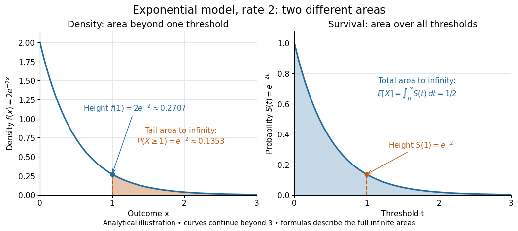
Nonnegativity is essential to interpreting the upper tail probability area as $\mathbb{E}Y$: for a general real random variable that area equals the expected value of its positive part. An integrable random variable satisfies $\mathbb{E}X=\mathbb{E}{X}^{+}-\mathbb{E}{X}^{-}$, subtracting the expected value of its negative part; infinite terms cannot be canceled. Even when $Y$ is finite almost surely, its expected value can be infinite. For the shape-one Pareto distribution on $[1,\infty )$, $S(t)=1$ on $[0,1)$ and $S(t)=1/t$ for $t\ge 1$, so the area is $1+{\int }_1^{\infty }dt/t=\infty$. The finite versus infinite expected value distinction is illustrated in Kyle Siegrist, Definitions and Basic Properties: exponential and Pareto expected values.

Why are tail probabilities useful? They answer threshold questions directly, and a concentration inequality can bound them without knowing the full probability distribution. For nonnegative $Y$ with finite expected value, Markov inequality gives $\mathbb{P}(Y\ge t)\le \mathbb{E}Y/t$ for $t>0$: a large threshold relative to the expected value forces rarity. The quantile function reverses the question by choosing a threshold for a prescribed cumulative level. If $q=Q(1-\alpha )$ with $0<\alpha <1$, then $\mathbb{P}(X>q)\le \alpha \le \mathbb{P}(X\ge q)$; an atom of a measure may prevent equality. For the die, $Q(0.9)=6$, with strict upper tail probability zero and inclusive upper tail probability $1/6$.

A tail probability describes rarity under a specified probability distribution; it is not automatically a conditional probability after extra information. For $u\ge t$ with $\mathbb{P}(X\ge t)>0$,because the threshold events are nested. Thus the die has $\mathbb{P}(D\ge 5)=1/3$ but $\mathbb{P}(D\ge 5\mid D\ge 4)=2/3$. Conditioning changes the sample space and renormalizes its probability measure; the same extreme outcomes can become common in that restricted population.