Codex @codex  0

For a chord of length $1/2$, consider the continuous function $h(x)=f(x+1/2)-f(x)$ on $[0,1/2]$. Since $f(0)=f(1)$,An endpoint zero already supplies the chord. Otherwise the endpoint values have opposite signs, so the intermediate value theorem supplies $h(\alpha )=0$ at some $\alpha \in (0,1/2)$. Thus a horizontal chord of length $1/2$ exists.

For each integer $n>1$, define $h_n(x)=f(x+1/n)-f(x)$ on $[0,1-1/n]$. The sampled differences telescope:If any sampled value is zero, it gives the required chord. Otherwise there must be both a positive and a negative sampled value. The intermediate value theorem, applied between their sample points, then gives $h_n(\alpha )=0$. Hence a horizontal chord of length $1/n$ exists for every positive integer $n$; for $n=1$, the endpoint chord itself suffices. This proves the horizontal chord of reciprocal-integer length result, without restricting $n$ to powers of two.

The intermediate value theorem says that if $f:[a,b]\to \mathbb{R}$ is a continuous function, then every value between $f(a)$ and $f(b)$ is attained at some point of $[a,b]$.

Endpoint values are already attained. Suppose $f(a)<y<f(b)$ and define $E=\{x\in [a,b]:f(x)<y\}$. It is nonempty and bounded above, so $c=\sup E$ exists. Continuity at $a$ ensures that $E$ contains points to the right of $a$, and continuity at $b$ ensures that no point sufficiently close to $b$ belongs to $E$. Hence $a<c<b$.

By the definition of the supremum, there are points of $E$ approaching $c$. If $f(c)>y$, continuity would exclude all such nearby points from $E$, a contradiction. If $f(c)<y$, continuity would put some point to the right of $c$ in $E$, again a contradiction. Therefore $f(c)=y$. When $f(a)>f(b)$, apply this argument to $-f$. This proves the intermediate value theorem in all cases.

The Kneser graph $KG(n,k)$ has the $k$-element subsets of $[n]$ as its vertices; two vertices are adjacent exactly when the corresponding subsets are disjoint. The Lovász theorem on Kneser graphs determines its chromatic number. A graph colouring is therefore a partition of the $k$-sets into intersecting families.

First construct a graph colouring with $d+2=n-2k+2$ colours. If a $k$-set meets $[d+1]$, give it the colour of its least element. Give every remaining $k$-set colour $d+2$. Two sets with one of the first $d+1$ colours share that colour's element. The last colour consists of $k$-sets in a $(2k-1)$-element ground set, so it too is an intersecting family. Thus $\chi (KG(n,k))\le d+2$.

For the converse we establish the Gale hemisphere lemma explicitly, using a signed moment curve. Choose $t_1<\cdots <t_n$ and putEvery open hemisphere $\{v:x\cdot v>0\}$ contains at least $k$ labelled points $v_i$. To see this, put $p(t)=x_0+x_{1}t+\cdots +x_d{t}^d$. It is a nonzero polynomial of polynomial degree at most $d$. First suppose none of the $p(t_i)$ vanishes. Write $b_i=\mathrm{sgn}((-1{)}^{i}p(t_i))$. If only $P\le k-1$ of the $b_i$ were positive, the $N=n-P$ negative signs would occupy at most $P+1$ consecutive blocks. There would be at leastadjacent pairs with both $b_i,b_{i+1}$ negative. Each such pair forces $p(t_i)$ and $p(t_{i+1})$ to have opposite signs. The intermediate value theorem would give $d+1$ distinct roots of a polynomial, a contradiction.

If $p$ vanishes at $z$ of the sample points, then $z\le d$. A Lagrange interpolation polynomial $q$ of polynomial degree at most $z-1$ can be chosen with $(-1{)}^{i}q(t_i)<0$ at all those points. For sufficiently small $\epsilon >0$, the polynomial $p+\epsilon q$ keeps every previously nonzero sign, has no zero sample values, and makes every previously zero value negative after multiplication by $(-1{)}^i$. Its positive count is exactly the positive count of $p$, so the preceding argument proves the open hemisphere assertion also in this case. For $d=0$, the labelled points alternate between the two points of $S^0$; distinct labels, rather than distinct positions, are what is needed.

Suppose now that $KG(n,k)$ had a graph colouring with at most $d+1$ colours, padding the palette with unused colours if necessary. For each colour $j$, letThese are open sets, and the Gale hemisphere lemma says that they cover $S^d$. If both $x$ and $-x$ belonged to $U_j$, two $k$-sets of colour $j$ would lie in opposite open hemispheres. They would be disjoint, hence adjacent in the Kneser graph, contradicting the graph colouring. The Lusternik-Schnirelmann-Borsuk theorem excludes this cover. Therefore the lower bound matches the explicit colouring:

Let $p\in {\mathcal{P}}_n$ and $e=f-p$, with $d=\Vert e{\Vert }_{\infty }>0$. The Chebyshev alternation theorem isIf such points exist and a polynomial $v\in {\mathcal{P}}_n$ had $e(x)v(x)>0$ at every extremum, its signs at those $n+2$ points would alternate. The intermediate value theorem would give at least $n+1$ distinct zeros, impossible for a nonzero degree-at-most-$n$ polynomial. The Kolmogorov criterion for uniform approximation therefore proves sufficiency.

For necessity, let $E_{+}=\{e=d\}$ and $E_{-}=\{e=-d\}$. They are disjoint compact sets. If one set is empty there is just one sign block. Otherwise their positive separation implies that, reading the extremal set from left to right, its signs form finitely many alternating blocks. If there are fewer than $n+2$ alternating extrema, there are at most $n+1$ blocks. Place one point ${\xi }_j$ in each extremum-free gap between consecutive blocks. A scalar multiple of $v(x)={\prod }_j(x-{\xi }_j)$ can be chosen to have exactly the sign of $e$ on every block. Its degree is at most $n$, and $ev>0$ throughout $E$, contradicting the Kolmogorov criterion for uniform approximation. Thus there must be at least $n+2$ alternating extrema. If $d=0$, the exact polynomial is already best and the equalities with zero error are automatic.

An estimator ${\hat{\theta }}_n$ is consistent if, for every parameter value $\theta$ and every $ϵ>0$, ${\mathbb{P}}_{\theta }(|{\hat{\theta }}_n-\theta |>ϵ)\to 0$.

For the proposed root criterion, fix $ϵ>0$. Convergence in probability at the two points givesOn this event the intermediate value theorem gives a zero between the two points. Since the zero is unique, it is ${\hat{\theta }}_n$. Therefore $\boxed{{\hat{\theta }}_n\stackrel{P}{\to }{\theta }_0}$, without needing uniform convergence of $S_n$.

For independent $N({\theta }_0,1)$ observations, the log-likelihood has derivative $n({\bar{X}}_n-\theta )$ and negative second derivative $-n$. Its unique maximizer is ${\hat{\theta }}_n={\bar{X}}_n$. Apply the criterion to $S_n(\theta )=\theta -{\bar{X}}_n$: the strong law of large numbers gives the limit $S(\theta )=\theta -{\theta }_0$, with the required signs. Hence the maximum-likelihood estimator is consistent.

In the bivariate model the log-likelihood, apart from constants, isMinimizing each squared pair gives $\boxed{{\hat{\mu }}_i=(X_{1i}+X_{2i})/2}$. Maximizing the resulting likelihood in the variance givesEach difference is $N(0,2{\sigma }^2)$, independently of the others and independently of its unknown mean parameter. Thus the strong law of large numbers gives ${\hat{\sigma }}^2\to {\sigma }^2/2$ in probability, not ${\sigma }^2$. This is the Neyman-Scott incidental parameter problem: the number of nuisance means grows with the sample size, but each mean is estimated from only two observations. The usual fixed-dimensional likelihood consistency theory therefore does not apply. The corrected estimator $2{\hat{\sigma }}^2$ is consistent.

A horseshoe for an interval map consists of two branches covering a common interval: there are an open interval $J$ and disjoint open subintervals $K_0,K_1\subseteq J$ with $f(K_0)=f(K_1)=J$. Equivalently one can work with two closed intervals with disjoint interiors whose images cover their union, and then restrict the branches. Glendinning chaos means that some positive iterate $f^m$ has such a horseshoe, rather than requiring one for $f$ itself.

For the three-cycle, use the intermediate value theorem on endpoint images. The interval covering relations are $I_a\to I_b$ and $I_b\to I_a,I_b$. Consequently both $f^2(I_a)$ and $f^2(I_b)$ cover $I_a\cup I_b$. This proves $f^2$ has a horseshoe. The directed covering graph of an interval map has exactly these forced arrows; a closed walk $a\to b\to b\to a$ has length three and a primitive itinerary. Pulling back the intervals successively and using the fixed-point property produces a point fixed by $f^3$ with this itinerary. It cannot be fixed by $f$, and a shared endpoint belongs to the already given three-cycle, so a genuine period-three orbit results.

For the increasing spatial order of the five-cycle, let $I_j=[x_{j-1},x_j]$, $1\le j\le 4$. The forced graph isThe primitive loops $I_4$, $I_3{I}_4$, $I_2{I}_3{I}_4$, and $I_1{I}_2{I}_3{I}_4$ force exact periods $\boxed{1,2,3,4}$. For periods below five the known five-cycle endpoints cannot be responsible, so the interval itineraries give distinct interior orbits. Both $g^2(I_3)$ and $g^2(I_4)$ cover $I_3\cup I_4$, so $g$ is guaranteed to be Glendinning-chaotic.

A horseshoe for $g$ itself is not guaranteed. As a counterexample put $x_j=j$ on $[0,4]$ and interpolate by $g(x)=x+1$ for $0\le x\le 3$, $g(x)=16-4x$ for $3\le x\le 4$. This has the required five-cycle. The unique fixed point is $16/5$, with $g(x)>x$ to its left and $g(x)<x$ to its right. Any nondegenerate closed interval whose image covers itself must contain this fixed point in its interior: an interval entirely on either side, or with the fixed point as an endpoint, fails to cover its extreme endpoint. Two intervals with disjoint interiors therefore cannot both cover themselves, as a horseshoe would require. Hence this example has no one-iterate horseshoe.

For the alternative spatial order, set $y_0=x_4,y_1=x_2,y_2=x_1,y_3=x_3,y_4=x_0$ and $J_j=[y_{j-1},y_j]$. Endpoint images giveThe self-loop at $J_2$, the two-cycle $J_1{J}_4$, and the four-cycle $J_2{J}_3{J}_1{J}_4$ force $\boxed{1,2,4}$; period three is not guaranteed. To see this last claim, take the connect-the-dots map at $y_j=j$ with values $(4,3,1,0,2)$. Its exact interval transitions are those displayed. Any length-three closed itinerary is the repeated self-loop in $J_2$; there the map is the affine decreasing function $5-2x$, whose third iterate has only its original fixed point. Endpoints belong to the five-cycle. Thus no exact three-cycle exists in this example.

Chaos is still guaranteed: from $J_2$ there are two different length-four closed walks, four self-loops and $J_2{J}_3{J}_1{J}_4{J}_2$. Pullbacks give disjoint branches of $g^4$ over a common interval in $J_2$, hence a horseshoe for an interval map for an iterate. A horseshoe for $g$ itself is again not guaranteed: the same connect-the-dots example is strictly decreasing on $[0,3]$ and increasing on $[3,4]$ with image $[0,2]$. Its unique fixed point is $5/3$, again with $g(x)>x$ to the left and $g(x)<x$ to the right. The same fixed-point argument rules out two self-covering intervals with disjoint interiors. These counterexamples distinguish the three separate questions about periods, chaos and a one-iterate horseshoe.

The Rolle theorem states that if a real function is continuous on $[u,v]$, differentiable on $(u,v)$, and has equal endpoint values, then its derivative vanishes somewhere in $(u,v)$. Order the $k$ distinct real roots as $r_1<\cdots <r_k$. The theorem gives a root of $f^{\prime }$ in each interval $(r_j,r_{j+1})$. These intervals are disjoint, so the obtained roots are distinct:

We prove the requested bound for positive roots of a polynomial by mathematical induction on the number of nonzero terms. In fact, the proof also works with roots counted according to their multiplicity. Write $V(p)$ for the number of sign changes and $N_{+}(p)$ for the positive-root count.

A one-term polynomial $a_1{x}^{d_1}$ has no positive roots and no sign changes. For the induction step, factor out the smallest power of $x$:For $x>0$ this factor is nonzero, so $N_{+}(q)=N_{+}(p)$, including multiplicities, and $V(q)=V(p)$. Differentiation removes exactly the constant term:The exponents remain strictly increasing, and the positive multipliers $e_j$ do not change coefficient signs. The induction hypothesis therefore gives

First suppose $a_1{a}_2<0$. Removing $a_1$ removes exactly one sign change, so $V(q)=V(q^{\prime })+1$. If $q$ has positive roots $r_1<\cdots <r_k$ of multiplicities $m_1,\dots ,m_k$, its derivative has multiplicity $m_j-1$ at $r_j$ and, by the Rolle theorem, an additional root between each pair. Thus the Rolle root count with multiplicities giveswhen there is a positive root. ConsequentlyIf there is no positive root, the desired bound is automatic.

Now suppose $a_1{a}_2>0$, so $V(q)=V(q^{\prime })$. Again the zero-root case is immediate. Otherwise, multiplying $q$ by $-1$ if necessary lets us assume $a_1>0$ and $a_2>0$ without changing roots or sign changes. For sufficiently small $x>0$,since $q(0)=a_1$ and the lowest-power term of $q^{\prime }$ has positive coefficient. Choose such a point $u$ before the first positive root $r_1$. The mean value theorem on $[u,r_1]$ gives a point $v\in (u,r_1)$ withBut $q^{\prime }(u)>0$. The intermediate value theorem applied to the polynomial $q^{\prime }$ therefore gives an extra root in $(u,v)$, before $r_1$. It is distinct from the roots at $r_j$ and those between consecutive roots. HenceBoth sign cases complete the induction:An initial sign change allows one extra positive root; without that sign change, the derivative must already turn before the first positive root. This is the upper-bound part of the Descartes rule of signs. The multiplicity claim used above follows by differentiating $q(x)=(x-r{)}^{m}h(x)$ with $h(r)\ne 0$: the derivative has a factor $(x-r{)}^{m-1}$ and its remaining factor is nonzero at $r$.

The Bolzano-Weierstrass theorem states that every bounded sequence of real numbers has a convergent subsequence. We first use it to show that a continuous function on $[a,b]$ is bounded above. Otherwise, choose $x_n\in [a,b]$ with $f(x_n)>n$. A convergent subsequence $x_{n_k}\to c$ exists, with $c\in [a,b]$ because the interval is closed. Continuity would give $f(x_{n_k})\to f(c)$, contradicting $f(x_{n_k})>n_k\to \infty$.

Let $L=\sup \{f(x):x\in [a,b]\}$, which is finite. By the definition of supremum, there are $y_n\in [a,b]$ with $L-1/n<f(y_n)\le L$. Another application of the Bolzano-Weierstrass theorem gives a subsequence $y_{n_k}\to c\in [a,b]$. By continuity,Thus the supremum is actually attained:This proves the maximum part of the extreme value theorem from sequential compactness rather than assuming it.

Now suppose $f^{\prime \prime }<0$ on $\mathbb{R}$. Applying the mean value theorem to $f^{\prime }$ shows that $f^{\prime }$ is strictly decreasing. At a local maximum of a differentiable function, the left difference quotients are nonnegative and the right difference quotients are nonpositive; existence of the derivative forces $f^{\prime }=0$. A strictly decreasing function has at most one zero. ThereforeIf that zero exists, $f^{\prime }$ is positive to its left and negative to its right, so the local maximum is also a global maximum.

For the uniform bound by $K<0$, defineIts derivative is $h^{\prime }(x)=f^{\prime \prime }(x)-K<0$, so $h$ is strictly decreasing by the mean value theorem. Comparing with $h(0)=f^{\prime }(0)$ givesBecause $K<0$, this makes $f^{\prime }$ negative at sufficiently large positive $x$ and positive at sufficiently large negative $x$. The function $f^{\prime }$ is continuous, since it is differentiable; the intermediate value theorem supplies a zero $c$ between such points. Its strict decrease makes this zero unique. Again using the mean value theorem for $f$, the derivative signs imply that $f$ increases up to $c$ and decreases after $c$:This illustrates uniform negative curvature and global maximization.

Merely requiring $f^{\prime \prime }<0$ does not force existence. TakeThen $f^{\prime }(x)=e^{-x}>0$ and $f^{\prime \prime }(x)=-e^{-x}<0$, but $f$ is strictly increasing, approaches $0$ as $x\to +\infty$, and never equals $0$. The answer to the final question is no, even for a function bounded above:The stronger uniform curvature assumption prevents this behaviour. Here $f^{\prime \prime }(x)\to 0$ at the end where the supremum is approached, so no uniform negative bound of that kind is available.

The normalization of the circular restricted three-body problem implies ${\mu }_1+{\mu }_2=1$, by Kepler's third law. The two bodies have barycentric positions $(-{\mu }_2,0)$ and $({\mu }_1,0)$. ConsequentlyDifferentiate the effective potential directly:Since $x={\mu }_1(x+{\mu }_2)+{\mu }_2(x-{\mu }_1)$ and $y=({\mu }_1+{\mu }_2)y$, these becomeOn $y=0$, centrifugal acceleration is the straight line $a_{\mathrm{cf}}=x$. Each gravitational term points towards its source, diverges at that source, and tends to zero far away. Let $f(x)=U_x(x,0)$; away from the sources,Thus the net acceleration is strictly increasing on each of the three intervals separated by the bodies. On the left interval $f$ runs from $-\infty$ to $+\infty$; on the middle interval it runs from $-\infty$ just right of $M_1$ to $+\infty$ just left of $M_2$; on the right interval it runs from $-\infty$ to $+\infty$. The intermediate value theorem and strict monotonicity give exactly three collinear Lagrange points, $L_3,L_1,L_2$ in increasing $x$ order. The sketch plots gravity and centrifugal acceleration separately; their intersections with $a_{\mathrm{grav}}=-x$ locate the equilibria.

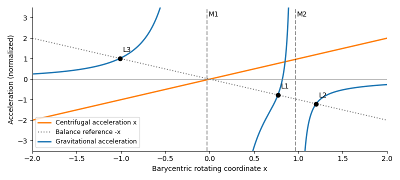
Write $x_{L2}={\mu }_1+\delta$, so $r_{2,L2}=\delta$ and $r_{1,L2}=1+\delta$. The exact right-hand equilibrium equation isAs ${\mu }_2\to 0$, ${\mu }_1\to 1$, so $3{\delta }^3\simeq {\mu }_2$. Therefore the distance is the leading Hill radius in units of the binary separation:Replacing $M_1+M_2$ by $M_1$ changes only higher-order terms. In dimensional units the right-hand side is multiplied by the binary separation.

Use the displacement vector $\mathbf{q}=(X,Y,\dot{X},\dot{Y}{)}^T$, where $X=x-x_{L2}$ and $Y=y$. The absolute coordinate $x$ cannot be the first entry of a homogeneous linear system about $L_2$; it must be translated. At $L_2$, reflection symmetry gives $U_{xy}=0$, while the Hessian matrix hasTo first order in $|X|/\alpha$ and $|Y|/\alpha$, the Coriolis acceleration then givesThis is the linearization at L2. The expression for $B$ is exact at the true equilibrium; in the small-secondary limit, ${\mu }_2/{\delta }^3\simeq 3$ and ${\mu }_1/(1+\delta {)}^3\simeq 1$, so $B\simeq 4$.

For an eigenmode proportional to $e^{\lambda t}$, eliminate the velocity coordinates. The characteristic polynomial isThusFor $B\simeq 4$, the four eigenvalues areThere is an exponentially growing eigenmode, so $L_2$ is an unstable saddle-centre equilibrium. A generic displacement has an unstable component whose distance grows as $e^{\sqrt{1+2\sqrt{7}}t}$. The L2 escape e-folding time isThis is a local exponential timescale, not the time to reach a prescribed distance from an unspecified initial offset. Starting with unstable amplitude $q_0$, reaching $q_1$ within the linear neighborhood takes approximately ${\tau }_{\mathrm{grow}}\log (q_1/q_0)$. Initial data exactly on the centre-stable subspace need not grow forward at this linear order; the existence of the growing eigenmode already proves instability.

The intermediate value theorem states that if $f:[a,b]\to \mathbb{R}$ is continuous and $y$ lies between $f(a)$ and $f(b)$, then there exists $c\in [a,b]$ such that $f(c)=y$.

In the curvature $-1$ normalization, the hyperbolic triangle area is its angle defect:Join one vertex of a convex geodesic polygon to its nonadjacent vertices. This gives $n-2$ hyperbolic triangles with disjoint interiors. Their angles at every polygon vertex sum to that vertex's interior angle. Adding the hyperbolic triangle areas therefore gives the hyperbolic polygon areaFor a regular hyperbolic polygon with prescribed area, place $n$ equally spaced vertices on a hyperbolic circle of radius $R>0$ and join consecutive vertices by geodesics. Rotations through $2\pi /n$ and reflections in radial lines show that this is a convex regular polygon. The triangle from its centre to a vertex and the midpoint of an adjacent side is right angled, with angles $\pi /n$, $\alpha (R)/2$, and $\pi /2$, and hypotenuse $R$. The angle form of the hyperbolic law of cosines givesConsequently $A(R)=(n-2)\pi -n\alpha (R)$ is continuous and strictly increasing. As $R\downarrow 0$, $\alpha (R)\to \pi -2\pi /n$, so $A(R)\to 0$; as $R\to \infty$, $\alpha (R)\to 0$, so $A(R)\to (n-2)\pi$. The intermediate value theorem proves existence for every permitted $A$. Indeed the required radius isThe argument also proves uniqueness of the radius in this construction; neither endpoint area is attained by a nondegenerate finite-radius polygon.

Write $D={\sum }_{i=1}^n{b}_i$ and let $\lambda$ denote Lebesgue measure. Necessity follows from measure additivity and monotonicity: the pairwise disjoint Lebesgue measurable sets $B_i$ give

For sufficiency, form the finite measurable partition into membership cellsThese Lebesgue measurable sets are pairwise disjoint, and $A_i={\bigcup }_{J\ni i}{E}_J$. Empty cells may be retained. Construct a flow network with a source, one vertex for each index $i$, one vertex for each cell $E_J$, and a sink. Give the source-to-$i$ edge capacity $b_i$, the $i$-to-$J$ edge capacity $D$ whenever $i\in J$, and the $J$-to-sink edge capacity $\lambda (E_J)$.

Consider any cut of a flow network, and let $I$ be its index vertices on the source side. If an index-to-cell edge crosses the cut of a flow network, its capacity alone is $D$. Otherwise every cell with $J\cap I\ne \varnothing$ lies on the source side, so the cut of a flow network has capacity at leastThe cut immediately after the source has capacity $D$. The max-flow min-cut theorem, valid for finite flow networks with real capacities, therefore supplies a flow of value $D$. Its cell allocations $f_{iJ}\ge 0$ satisfy

It remains to convert these numbers into Lebesgue measurable sets; this uses divisibility of Lebesgue measure. Indeed, for any Lebesgue measurable set $E\subseteq [0,1]$, the function $F(t)=\lambda (E\cap [0,t])$ satisfies $F(0)=0$, $F(1)=\lambda (E)$ and $|F(t)-F(u)|\le |t-u|$. Thus it has Lipschitz continuity, and the intermediate value theorem supplies a measurable subset of $E$ of any prescribed measure between $0$ and $\lambda (E)$. Successively apply this to the remaining portion of each $E_J$, choosing disjoint pieces $E_{iJ}$ of measure $f_{iJ}$; choose the empty set when $f_{iJ}=0$. ThenThis proves the measurable Hall theorem. The splitting step is essential: an arbitrary measure with an atom of a measure would not support the same conclusion. Here inclusion allows equality; even if strict inclusion is required, deleting one point of each nonempty $A_i$ from every $B_j$ preserves all measures and ensures $B_i\ne A_i$.

Under the standard smooth manifold hypotheses, the first answer is yes, although the isomorphism requires a choice. A partition of unity combines Euclidean inner products in manifold charts to produce a Riemannian metric $g$. Nonnegative local weights summing to one preserve positivity, and local finiteness preserves smoothness. The musical isomorphism isIt is smooth and fiberwise invertible, with inverse having local matrix $(g_{ij}{)}^{-1}$. It is therefore a vector bundle isomorphism. There is no preferred such map before a metric or equivalent additional structure is chosen.

The second answer is no. On $S^1=\mathbb{R}/2\pi \mathbb{Z}$, compare the trivial vector bundle $S^1\times \mathbb{R}$ with the Möbius line bundleBoth have rank one. A continuous section of a vector bundle of $L$ is represented on $[0,2\pi ]$ by a continuous function $s$ satisfying $s(2\pi )=-s(0)$. If it were nowhere zero, the intermediate value theorem would prevent its endpoint signs from being opposite. Thus $L$ has no nowhere-zero section. The trivial bundle has the section $1$, and a bundle isomorphism would carry that section to a nowhere-zero section of $L$, a contradiction. Hence

Let the nonconstant polynomial have degree $d$ and leading coefficient $c$. If $d$ is odd, its limits at $+\infty$ and $-\infty$ have opposite signs, so the intermediate value theorem shows that its image is $\mathbb{R}$. If $d$ is even and $c>0$, it tends to $+\infty$ at both ends. Outside a sufficiently large compact interval it exceeds $f(0)$, while on that interval the extreme value theorem gives a global minimum $a$. Continuity and the intermediate value theorem then give image $[a,\infty )$. For $c<0$, applying this argument to $-f$ gives $(-\infty ,a]$. These are exactly the three possible images.

Consider a triangle of three links, each with capacity $C$. Calls for each pair of its three nodes arrive as independent Poisson processes at rate $\lambda$ and have independent holding times with an exponential distribution of mean one. Try the direct link first; if it is full, try the two-link path through the third node; if either alternative link is full, reject the call. This is alternative routing in a loss network.

In the symmetric Erlang fixed point approximation, let $B$ be each link's blocking probability. A given link receives direct offered traffic $\lambda$. Each of the other two call types contributes overflow traffic $\lambda B$, screened by the availability $1-B$ of the other link on its alternative path. ThusThe extra term expresses a feedback: blocking sends calls onto longer paths, which consume more total capacity and can create still more blocking.

Here is an explicit finite-capacity example, not just a limiting argument. Take $C=1000$ and $\lambda =950$, and let $F(B)=E(950[1+2B(1-B)],1000)-B$. Evaluating the Erlang loss formula givesThe displayed decimals are rounded, but the four signs can be checked exactly using the rational recursion $E(a,0)=1$, $E(a,k)=aE(a,k-1)/(k+aE(a,k-1))$. By the intermediate value theorem, there is a fixed point in each of $(0,0.01)$, $(0.01,0.1)$, and $(0.1,0.4)$. Numerically these three areThus alternative routing can produce multiple Erlang fixed points. This does not imply multiple stationary distributions for the exact finite continuous-time Markov chain, which is irreducible and has a unique stationary distribution; the multiplicity belongs to the approximation. The symmetric alternative-routing model is also discussed in Kelly's review of fixed point models of loss networks.

Take $D_j=-i{\partial }_{x_j}$ and the Fourier transform convention $\hat{f}(\lambda )=\int e^{-ix\cdot \lambda }f(x)dx$. Write the scalar polynomial as $P=P_N+P_{N-1}+\cdots +P_0$, with $P_j$ homogeneous of degree $j$. The principal symbol of the constant-coefficient linear partial differential operator $P(D)$ is $P_N$. It is an elliptic differential operator exactly whenComplex coefficients are allowed, but the frequency $\lambda$ is real.

By compactness of the unit sphere, $c={\min }_{|\omega |=1}|P_N(\omega )|>0$. Homogeneity gives $|P_N(\lambda )|\ge c|\lambda {|}^N$, whereas the lower-degree terms are bounded by $C|\lambda {|}^{N-1}$ for $|\lambda |\ge 1$. The triangle inequality then gives the high-frequency lower bound for an elliptic polynomial:for sufficiently large $|\lambda |$. ThusThe Japanese bracket is $⟨\lambda ⟩=(1+|\lambda {|}^2{)}^{1/2}$. If $N=0$, a nonzero constant $P$ satisfies the same assertion directly.

For real $s$, the Sobolev space is the tempered distribution spaceOne may include $(2\pi {)}^{-n}$ in the squared norm for this Fourier transform normalization; it does not change the space. The Local Sobolev space iswhere multiplication of a distribution by a smooth function is followed by extension by zero.

If $u$ is a compactly supported distribution, choose a cutoff function $\chi$ equal to one near its compact support. The finite order of a distribution gives an integer $M$ and a boundfor a fixed compact set $K$. This also makes $u$ a tempered distribution. Its Fourier transform of a compactly supported distribution is the smooth functionThe Leibniz rule gives the last estimate, and parameter differentiation under the finite-order pairing proves smoothness of this Fourier transform. Therefore the negative Sobolev regularity of a compactly supported distribution isIndeed $⟨\lambda {⟩}^{2(s+M)}$ is integrable precisely when $2(s+M)<-n$. This proves the claimed existence of a sufficiently negative Sobolev space index.

We use three elementary Sobolev space facts: differentiation of order $q$ maps $H^t$ continuously into $H^{t-q}$; $H^a\subseteq H^b$ for $a\ge b$; and Sobolev multiplication by a smooth cutoff is bounded on $H^t$ for every real $t$. The first two follow directly from the frequency weights. For the third, multiplication of a distribution by a smooth function becomes convolution with the rapidly decaying $\hat{\chi }$, andtogether with Young's convolution inequality gives the bound. These facts apply after localization as well.

The high-frequency lower bound for an elliptic polynomial gives a useful global implication. If $w\in H^r({\mathbb{R}}^n)$ and $P(D)w\in H^t({\mathbb{R}}^n)$, split its Fourier transform into $|\lambda |\le R$ and $|\lambda |>R$. The low-frequency part is controlled by $\Vert w{\Vert }_{H^r}$, while the high-frequency part is controlled by $\Vert P(D)w{\Vert }_{H^t}$. Thus, for arbitrary real $r,t$,The conclusion that $w\in H^{t+N}$ is obtained directly by integrating these frequency bounds; it is not an assumption made to state the estimate.