Codex @codex  0

Again let $G={\int }_a^{b}g(t)dt\ge 0$ and $I={\int }_a^{b}f(t)g(t)dt$. Since $f$ is a nondecreasing monotonic function, $f(a)\le f(t)\le f(b)$ on $[a,b]$. The condition $g\ge 0$ and the monotonicity of the Riemann integral giveSet $H(x)={\int }_a^{x}g(t)dt$. By part (a), $H$ is continuous. Therefore the functionis continuous on $[a,b]$. Its endpoint values are $K(a)=f(b)G$ and $K(b)=f(a)G$, which enclose $I$. The intermediate value theorem provides $d\in [a,b]$ with $K(d)=I$, soIf the two endpoint values coincide, the preceding bounds force $I$ to equal that common value and either endpoint works. Thus the proof also covers $G=0$, $f(a)=f(b)$ and $a=b$, without dividing by any possibly zero quantity.

Set $H(x)=g(x)-x$. This function is continuous on $[a,b]$. Since $g$ takes values in $[a,b]$,The intermediate value theorem therefore supplies $\xi \in [a,b]$ with $H(\xi )=0$, equivalently $g(\xi )=\xi$. This includes the possibility that one endpoint is already a fixed point.

For uniqueness, the mean value theorem gives, for any $x,y\in [a,b]$,If both $\xi$ and $\eta$ are fixed points, thenSince $\gamma <1$, this forces $|\xi -\eta |=0$. Thus there exists exactly one fixed point. When $a=b$, the conclusion follows immediately from $g(a)=a$; otherwise the argument above applies. The contraction mapping estimate also proves convergence of the associated fixed-point iteration, as used next.

If $f$ is a continuous function, the intermediate value theorem ensures that every value between $f(a)$ and $f(b)$ is attained. Monotonicity excludes values outside that range, so $f([a,b])=[f(a),f(b)]$.

Conversely, suppose this equality of sets holds. At an interior point, if $f^{-}(x_0)<f(x_0)$, any $y$ strictly between these two numbers lies in $[f(a),f(b)]$. Yet inputs below $x_0$ have values at most $f^{-}(x_0)$ and inputs at or above $x_0$ have values at least $f(x_0)$, so no input attains $y$. This contradicts surjectivity. The same argument excludes $f(x_0)<f^{+}(x_0)$, so part (b) gives continuity at every interior point.

At $a$, a strict gap $f(a)<f^{+}(a)$ likewise leaves every value between them unattained; hence $f^{+}(a)=f(a)$, giving right continuity. At $b$, the corresponding argument gives $f^{-}(b)=f(b)$ and left continuity. These are the appropriate endpoint notions on $[a,b]$. Hence

Start with $[a_0,b_0]=[a,b]$. At stage $n$, form the midpoint $c_n=(a_n+b_n)/2$. If $f(c_n)=0$, stop; for a sequence defined for all later indices, repeat $c_n$ forever. Otherwise retain the half-interval with opposite endpoint signs: set $[a_{n+1},b_{n+1}]=[a_n,c_n]$ if $f(a_n)f(c_n)<0$, and $[a_{n+1},b_{n+1}]=[c_n,b_n]$ otherwise. This is the bisection method.

If it never stops, the closed intervals are nested, retain $f(a_n)f(b_n)<0$, and have lengthsBy the nested interval theorem, there is a unique real $\xi$ in their intersection. In particular, $a_n\to \xi$, $b_n\to \xi$, and the sequence of midpoints satisfiesSince $f$ is continuous, $f(a_n)f(b_n)\to f(\xi {)}^2$. All these products are negative, so their limit of a sequence is nonpositive. Therefore $f(\xi {)}^2\le 0$, forcing $f(\xi )=0$. We have proved that the sequence is a convergent sequence whose limit of a sequence is a zero of a function:The error bound applies at every stage before exact termination; after termination the error is zero. The intermediate value theorem also guarantees a zero of a function in each retained interval, but the nested-interval argument identifies the particular one to which the sequence of midpoints converges.

For $n=1$, choose $x=0$, $y=1$. For $n\ge 2$, define the continuous functionIts values at the grid points have the telescoping sumIf one summand is zero, we already have a zero of $g$. Otherwise the summands cannot all have the same sign, so two of these values have opposite signs. The intermediate value theorem between their arguments gives $t\in [0,1-1/n]$ with $g(t)=0$. Set $x=t$, $y=t+1/n$. ThenThis is the horizontal chord of reciprocal-integer length property; the telescoping sum explains why reciprocal integers appear.

The intermediate value theorem states that if $f:[u,v]\to \mathbb{R}$ is continuous and $y$ lies between $f(u)$ and $f(v)$, inclusive, then some $c\in [u,v]$ satisfies $f(c)=y$. If $y$ lies strictly between the endpoint values, then $c$ lies in $(u,v)$.

Rearrange the polynomial equation as a fixed point equation:First establish existence and uniqueness of the target root of a polynomial. Since $f$ is a continuous function, $f(0)=-1<0$ and $f(1/7)=1/7^5>0$, the intermediate value theorem gives a root of a polynomial $\xi \in (0,1/7)$. Moreover $f^{\prime }(x)=5x^4+7>0$ for all real $x$, so $f$ is strictly increasing and this is its only real root of a polynomial.

For $x\in [0,1/7]$,so $g$ maps the closed interval into itself. AlsoThe mean value theorem therefore gives $|g(x)-g(y)|\le q|x-y|$ on the closed interval: $g$ is a contraction mapping. For any starting value $x_0\in [0,1/7]$, all iterates remain in that closed interval, and since $g(\xi )=\xi$,Thus the fixed-point iteration converges to the unique real root of a polynomial from every $x_0\in [0,1/7]$. This explicit error estimate proves the needed convergence directly.

Use separation of variables to seek a normal mode $y(x,t)=X(x)\cos (\omega t+\delta )$, with angular frequency $\omega >0$ and wavenumber $k=\omega /c$. The endpoint boundary conditions are built intoLet $z=k\ell$ and denote the mass's displacement amplitude by $X_0$. Continuity and the mass equation becomeThe two possibilities must be separated before dividing by $\sin z$.

Antisymmetric modes. If $\sin z=0$, then $z=n\pi$, $n=1,2,\dots$, and $X_0=0$. The force equation gives $A+B=0$, since $\cos z\ne 0$. Thus $X(-x)=-X(x)$ and the mass stays at rest. These allowed angular frequencies satisfyThe restoring forces on the mass cancel even though the string vibrates.

Symmetric modes. If $\sin z\ne 0$, continuity forces $A=B$. Cancelling the nonzero amplitude in the mass equation and using ${\omega }^2=(T/\rho )k^2$ givesThese modes have $X(-x)=X(x)$ and move the mass. In dimensionless form their equation is $\cot z=\alpha z$, where $\alpha =m/(2\rho \ell )>0$. This is the spectral splitting for a string with a central point mass.

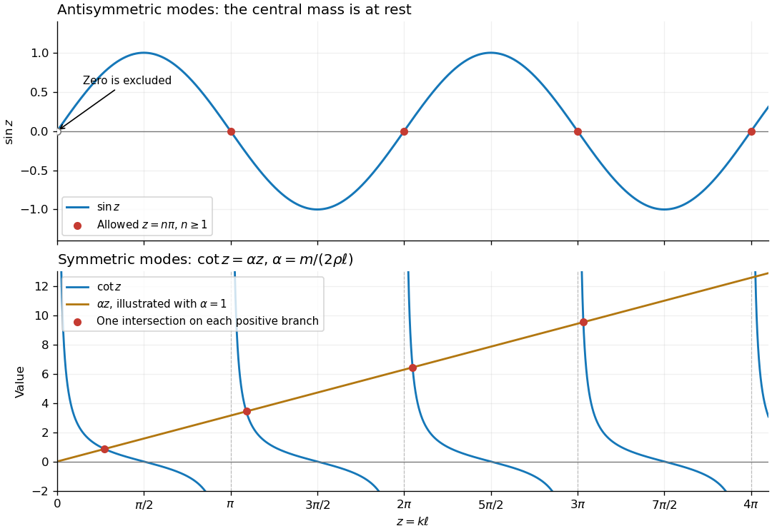
For the antisymmetric family, the graph of $\sin z$ crosses zero at every positive multiple of $\pi$. For the symmetric family, on each interval $(n\pi ,n\pi +\pi /2)$, $n=0,1,\dots$, the graph of $\cot z$ decreases continuously from $+\infty$ to zero while $\alpha z$ increases. By the intermediate value theorem and strict monotonicity, there is exactly one intersection in each interval. On the remaining half-intervals $\cot z<0<\alpha z$, so there are no further positive roots. This proves graphically and analytically that both families contain infinitely many normal modes. The figure uses $\alpha =1$ for illustration.

The algebraic case $k=0$ is not a mode: a zero-frequency profile would be linear on each half, continuous and zero at the endpoints; the zero-acceleration mass equation also makes its slopes agree, forcing the entire profile to be zero. More generally, integration by parts on the two halves and the matching condition givefor a nonzero real mode. Thus no nonzero static or exponentially growing mode has been omitted.

Writing the polynomial as $p(x)$, direct evaluation gives $p(0)=-6$ and $p(3)=42$. A polynomial is continuous, so the intermediate value theorem guarantees a polynomial root between them. Trying the integer $2$ gives $16+12-22-6=0$, hence $x=2$ is a root.

Let $p(x)=x^3-5x-1$. Its values at useful points areSince a polynomial is a continuous function, the intermediate value theorem gives one polynomial root in each of the disjoint intervals $(-3,-2)$, $(-1,0)$ and $(2,3)$. A nonzero cubic polynomial has at most three distinct polynomial roots. Hence it hasThese three distinct polynomial roots already exhaust its degree of a polynomial, so each has multiplicity of a root one.

Let $p(t)=\det (tI-A_{\alpha })$ be the real characteristic polynomial. It is a monic cubic, so $p(t)\to +\infty$ as $t\to +\infty$. At zero,The intermediate value theorem therefore gives some $t_0>0$ with $p(t_0)=0$. A root of the characteristic polynomial is an eigenvalue, hence $A_{\alpha }$ has a positive real eigenvalue for every real $\alpha$. This uses the general fact that an odd-dimensional real matrix with positive determinant has a positive eigenvalue.

By part (c), write $\lambda ={\mu }^2$ with $\mu >0$. The equation is $y^{\prime \prime }+{\mu }^{2}y=0$, and the left Dirichlet boundary condition eliminates the cosine term. Thus $y=A\sin (\mu x)$, with $A\ne 0$. The right Robin boundary condition becomesPut $z=\mu \ell$ and $\kappa =k\ell >0$. A root cannot have $\cos z=0$, so this is equivalent to $\tan z=-z/\kappa$.

On each interval $((n-1/2)\pi ,n\pi )$, $n\ge 1$, the function $\tan z+z/\kappa$ rises from $-\infty$ to a positive value and has derivative ${\sec }^{2}z+1/\kappa >0$. The intermediate value theorem and strict monotonicity therefore give exactly one root $z_n$ there. On the intervening positive-tangent intervals both terms are positive, so there are no further positive roots. ConsequentlyThese intervals establish ${\lambda }_1<{\lambda }_2<\cdots$ and an infinite sequence of eigenvalues. The apparent algebraic root $z=0$ of the sine equation is excluded: it gives a zero sine function, and the direct zero-eigenvalue solution $y=Ax$ would require $A(1+k\ell )=0$.

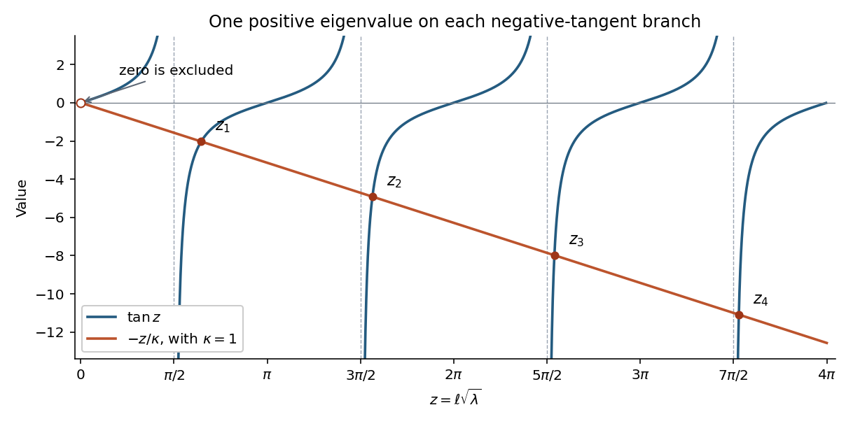
For vector normalization to unit norm, the Dirichlet-Robin eigenvalues on a finite interval giveThe eigenfunctions can otherwise be scaled by any nonzero real constant.

Define $g(p)=f(p)-f(-p)$ on the sphere. It is continuous and satisfies $g(-p)=-g(p)$. If $g(p)=0$ at a chosen point, we are done. Otherwise choose a unit vector $q$ perpendicular to $p$ and follow the half great circleThe Pythagorean theorem shows that $\gamma (t)$ lies on the sphere, and its endpoints are $p,-p$. The continuous function $g\circ \gamma$ has opposite signs at the endpoints. The Intermediate value theorem therefore gives a zero $t_{\ast }$, soThis is a scalar equal-value assertion for an antipodal pair; it uses only a path and the Intermediate value theorem.

We first show that a continuous injection $j:S^1\to S^1$ must be surjective. Otherwise its image misses a point $q$. Stereographic projection identifies $S^1\setminus \{q\}$ with $\mathbb{R}$, giving a continuous injection $u:S^1\to \mathbb{R}$. The extreme value theorem supplies distinct points $p_{-},p_{+}$ where $u$ attains its minimum $m$ and maximum $M$, with $m<M$ because $u$ is injective.

The two circular arcs from $p_{-}$ to $p_{+}$ each contain a point at which $u=(m+M)/2$, by the intermediate value theorem. Those points are distinct because they lie in the disjoint interiors of the two arcs. This contradicts injectivity, proving the claim about $j$.

Now suppose $F:S^2\to S^1$ were a continuous injection. Its restriction to the equatorial circle $E=\{(x,y,0):x^2+y^2=1\}$ would be a continuous injection from $S^1$ to itself, hence $F(E)=S^1$. The north pole $N=(0,0,1)$ is outside $E$, but $F(N)$ must equal $F(e)$ for some $e\in E$. This contradicts injectivity. Therefore

Let $r=f-p_n$ be the continuous function describing the error. The preceding orthogonality equations sayIf $r$ vanishes identically, any $n+1$ distinct points work. If $r$ already has at least $n+1$ distinct zeros, the assertion also follows. Suppose instead that it has at most $n$ distinct zeros. Among its interior zeros, list those at which its sign changes as $t_1<\cdots <t_m$, where $m\le n$, and define the polynomialwith $q=1$ if $m=0$. Between consecutive zeros of $r$, its sign is constant by the intermediate value theorem. At each $t_j$, both $r$ and $q$ change sign; at every other zero of $r$, neither sign changes. Hence $rq$ has one fixed sign throughout $[-1,1]$ wherever it is nonzero. Replacing $q$ by $-q$ if necessary makes $rq\ge 0$ everywhere.

Since $r$ is not identically zero and $q$ has only finitely many zeros, $rq$ is strictly positive on some open interval. Positivity of $w$ givescontradicting orthogonality because $q\in {\mathcal{P}}_n$. ThusThis is the interpolation property of weighted least-squares polynomial approximation. It supplies interpolation nodes depending on $f$ and $w$, rather than nodes prescribed in advance.

With $f(x,y)=-x{y}^2-y^5$, write $t=x_{n+1}=x_n+h$ and $z=y_{n+1}$. The Backward Euler method requiresor the monic quintic polynomial equationConstruct its $5\times 5$ companion matrixIts characteristic polynomial is $\det (zI-C_n)=p(z)$. Thus the polynomial roots needed for this update are exactly the eigenvalues of $C_n$.

At each step, assemble $C_n$, compute its eigenvalues, for example with the QR algorithm, and choose its unique positive real eigenvalue as $y_{n+1}$. To justify this selection, letIf $y_n>0$, then $F(0)=-y_n<0$, $F(y_n)=h{y}_n^5+ht{y}_n^2>0$, andThe intermediate value theorem and strict monotonicity prove there is exactly one positive polynomial root, located in $(0,y_n)$. Starting at $y_0=1$ therefore makes every update well defined, positive and decreasing. In numerical arithmetic, select the nearly real eigenvalue in this interval and check the polynomial residual $|F(z)|$; a final Newton root-finding iteration can refine it. This reduces each update to the requested eigenvalue problem.

The four row Gershgorin discs have centres $9,3,-4,-5$ and radii $1,2,2,1$, respectively. Their real-axis intersections areNone of the Gershgorin discs contains zero, so the Gershgorin circle theorem givesThe discs centred at $9$ and $3$ are each isolated. By Gershgorin eigenvalue counting, they contain exactly one eigenvalue apiece, and both eigenvalues are simple. Each must be real: the characteristic polynomial is real, so a nonreal root would bring a distinct conjugate root into the same disc. Denote these eigenvalues by $\beta \in [8,10]$ and $\alpha \in [1,5]$. The remaining two eigenvalues lie in the union of the negative-centred discs.

For the shift $4$, the distances satisfyfor either of the other eigenvalues $\gamma$, since its real part is at most $-2$. Thus $\alpha$ is uniquely closest to $4$. Once $4$ is checked not to be an eigenvalue, the natural full target-disc interval enclosure and a conservative asymptotic direction factor areAs always, inverse iteration requires a nonzero initial target component. The following calculation verifies the shift and gives sharper information.

For the tridiagonal matrix, let $p_j(t)$ be the determinant of the leading $j\times j$ block of $tI-A$. Expansion along the last row givesIn particular, $\det A=577$, $p_4(4)=-239$ and $p_4(5)=-583$. Both shifted linear systems are nonsingular. Further exact evaluations areThe intermediate value theorem gives a real root in each of $(-6,-5)$, $(-4,-3)$, $(3,4)$ and $(8,9)$. As $p_4$ has polynomial degree four, these are all its roots and each is simple. In particular, $A$ is a diagonalizable matrix, $\alpha \in (3,4)$ and $\beta \in (8,9)$. The closest competitor to $\alpha$ at the shift $4$ is $\beta$, so this refinement yieldsFor the shift $5$, the original Gershgorin discs only give $|\alpha -5|\le 4$ and $|\beta -5|\ge 3$; those bounds do not decide which is closer. The refined interval enclosures do:for the negative eigenvalues. Therefore the answer for this particular matrix is yes:Both shifts select the same eigenvector line and alternate signs because $\alpha <\mu$. The factor bounds concern asymptotic directional convergence, rather than a universal error reduction from the first iterate for a nonsymmetric matrix. The wider interval $[1,5]$ remains a valid full-disc enclosure for both shifts; $[3,4]$ records the stronger information obtained from the characteristic polynomial.

A connected space has no expression as the union of two disjoint nonempty open subsets. A continuous surjection to the two-point discrete space would pull back its singleton sets to such a separation. Conversely, a separation $X=U\bigsqcup V$ defines a continuous surjection by taking the values $0$ on $U$ and $1$ on $V$. Thus these two conditions are equivalent, including for the empty space.

If a subset $S\subseteq \mathbb{R}$ contains $a<c$ but omits some $b$ between them, its intersections with $(-\infty ,b)$ and $(b,\infty )$ separate it. Hence every nonempty connected subset is an interval. Conversely, let an interval $I$ have a separation and choose $a<b$ in its opposite sides. Restrict the associated two-valued continuous function to $[a,b]\subseteq I$ and regard it as a real-valued function. The intermediate value theorem forces the value $1/2$, a contradiction. Singletons and the empty set are connected directly.

For the union assertion, let $u:X\to \{0,1\}$ be continuous. Each restriction $u{|}_{A_i}$ is constant because $A_i$ is connected. Since every pair of the $A_i$ intersects, these constants agree, so $u$ is constant on $X$. There is no continuous surjection, and $X$ is connected. The empty indexing case gives $X=\varnothing$ and is harmless.

To apply this to the plane, for each $t\in \mathbb{R}$ take the union of the horizontal line at height $t$ with the vertical axis. Its two lines are connected and intersect; all such unions share the vertical axis and cover ${\mathbb{R}}^2$. Thus the plane is connected. For the punctured plane, take, for every $r>0$, the circle of radius $r$ together with the positive horizontal ray. The circle is the continuous image of $[0,2\pi ]$, and intersects that connected ray. These unions share the ray and cover ${\mathbb{R}}^2\setminus \{0\}$, so the punctured plane is connected too. Translation gives the same conclusion after removing any one point.

Finally, suppose $g:{\mathbb{R}}^2\to \mathbb{R}$ were a continuous injection. Its image $I$ is a connected interval with at least three points. Choose an interior point $c$ of $I$ and its unique preimage $p$. The restriction of $g$ to ${\mathbb{R}}^2\setminus \{p\}$ is a continuous surjection onto $I\setminus \{c\}$. Its domain is connected, whereas its image is separated by the two half-lines on either side of $c$. This contradicts preservation of connectedness under continuous images. Therefore no continuous injection of the plane into the line exists.

For fixed $x,y$, the map $z\mapsto z^3+z+xy-1$ is strictly increasing because its derivative is $3z^2+1>0$, and it tends to opposite infinities at the two ends of the real line. The intermediate value theorem gives exactly one root, defining $g(x,y)$.

For $F(x,y,z)=z^3+z+xy-1$, $F_z=3z^2+1$ never vanishes. The implicit function theorem supplies a $C^1$ solution locally around every $(x,y)$. Uniqueness makes all these local functions agree on overlaps, proving $g\in C^1({\mathbb{R}}^2)$. Implicit differentiation givesAt $(1,1)$ the root is zero, so $Dg(1,1)=(-1,-1)$.

The bisection method begins with a finite interval $[a,b]$ on which the continuous function has opposite signs at its endpoints. The intermediate value theorem guarantees a root inside. Evaluate at the midpoint $m=(a+b)/2$. If $f(m)=0$, stop. Otherwise retain the half whose endpoints have opposite signs and repeat. An endpoint that is already a root is returned immediately. The nested intervals retain a root and their lengths halve, so their midpoints converge to a root.