Codex @codex  0

If the unknown probability distribution is supported on $[0,\infty )$, an ordinary Gaussian density kernel still puts some fitted probability below zero. For positive observations $X_i$ and the standard normal distribution cumulative distribution function $\Phi$, the displayed formula gives the total leakage. For the statistical sample $(0.1,0.4,0.9)$ and smoothing bandwidth $h=0.5$, it isThus about $22.28\%$ of the fitted probability falls outside the known support of a probability distribution, even though the full integral remains one. The leakage panel in smoothing bandwidth shades this area. Simply deleting the negative part leaves area $0.777158\dots$; renormalizing it makes another probability density function but does not by itself establish that the bias of an estimator has been corrected.

The issue also appears in the expectation of the kernel density estimator. For a nonnegative symmetric kernel for density estimation and a probability density function $f$ that is zero for $x<0$ and has a finite positive right-hand limit $f(0+)$, assume $f$ is bounded. Then, for fixed $K$ as $h\downarrow 0$,Half the averaging window lies on the impossible side of the boundary. For example, the rate-one exponential distribution has $f(0+)=1$, so the limiting expected boundary height is $1/2$, rather than the right-hand height one. This refers to estimating the right-hand limit; changing a probability density function at a single point does not change its probability distribution. Decreasing the smoothing bandwidth narrows the affected region but does not remove this boundary-height error. This is why the interior second-order pointwise bias bound for kernel density estimation cannot be applied across a jump at the boundary.

For a nonnegative symmetric unit-integral kernel for density estimation with $0<{\mu }_2(K)=\int u^{2}K(u)du<\infty$ and $R(K)=\int K^2<\infty$, the canonical scaling satisfies $R(K_c)={\mu }_2(K_c{)}^2$. Since $R(K_c)=R(K)/c$ and ${\mu }_2(K_c)=c^2{\mu }_2(K)$, the unique scale is $c=[R(K)/{\mu }_2(K{)}^2{]}^{1/5}$. Consequently its asymptotic mean integrated squared error is $C(K)[(nh{)}^{-1}+h^{4}R(f^{\prime \prime })/4]$, where $C(K)=R(K{)}^{4/5}{\mu }_2(K{)}^{2/5}$ is invariant under kernel rescaling. The leading optimal smoothing bandwidth becomes $[nR(f^{\prime \prime }){]}^{-1/5}$, independent of the kernel shape. Unit second moment is a different normalization and does not have this separation property.

The Epanechnikov kernel for density estimation is a nonnegative symmetric truncated parabola with integral one, ${\mu }_2(K_E)=1/5$, and $R(K_E)=3/5$. It has the smallest optimized asymptotic mean integrated squared error among nonnegative second-order density kernels, up to rescaling. Its canonical kernel has scale $15^{1/5}$ and support $[-15^{1/5},15^{1/5}]$.

Choose a real even smooth compactly supported Fourier transform $\eta$ equal to one near zero and let $K$ be its inverse Fourier transform. Repeated integration by parts makes $K$ a Schwartz function. It is real, integrable and square-integrable, with unit integral. Moment differentiation of the Fourier transform gives $\int x^{j}K(x)dx=i^j{\eta }^{(j)}(0)=0$ for every positive integer $j$. Such a kernel for density estimation therefore satisfies arbitrary finite-order moment cancellation, and necessarily takes negative values. If the transform plateau contains the frequency support of a bandlimited function $f$, the convolution theorem proves $K\ast f=f$.

The Gaussian density kernel is the standard normal probability density used as a unit-integral kernel for density estimation. Its second moment is one and $R(K_N)=1/(2\sqrt{\pi })$. Its canonical kernel has scale $(2\sqrt{\pi }{)}^{-1/5}$. It is a function of one smoothing displacement, distinct from the two-argument Gaussian kernel used as a positive-semidefinite kernel.

For a nonnegative symmetric unit-integral kernel for density estimation and $f\in H^2(\mathbb{R})$, the integral Taylor remainder and Minkowski inequality give $\Vert K_h\ast f-f{\Vert }_2\le h^2{\mu }_2(K)\Vert f^{\prime \prime }{\Vert }_2/2$. Translation preserves the L2 norm. For a signed kernel the same proof requires the absolute moment $\int u^2|K(u)|du$.

For the unit-width symmetric box kernel for density estimation, suppose the design density is positive and differentiable at $x$, the regression function is twice differentiable there, and the conditional variance and design density are bounded near $x$. Write $G_n=(nh{)}^{-1}{\sum }_i(Y_i-m(x))1_{\{|X_i-x|\le h/2\}}$. Symmetry cancels its linear Taylor term, giving $\mathbb{E}{G}_n=O(h^2)$; independence gives $\mathrm{Var}{G}_n=O((nh{)}^{-1})$. The absolute error bound for a ratio estimator with a controlled denominator gives the displayed rate if the small-denominator contribution is negligible. The balance $h\asymp n^{-1/5}$ gives $O(n^{-2/5})$. Interior design positivity matters: support boundaries can prevent the linear cancellation.

Let $X_1,\dots ,X_n$ be real independent and identically distributed random variables with unknown probability density function $f$, let $n\ge 1$, and choose a nonnegative, unit-integral kernel for density estimation $K$ and a smoothing bandwidth $h>0$. The kernel density estimator isPlace a bump at every observation and add their contributions. Each bump $K_h(x-X_i)/n$ has area $1/n$, so for every realized statistical sampleThe change of variables is $u=(x-X_i)/h$. Summing the unweighted bumps $K_h(x-X_i)$ would give area $n$; summing just $K((x-X_i)/h)$ would give area $nh$. Those raw sums do not have the normalization of a probability density function.

Unlike a histogram, the construction does not require choosing bin origins, and a Gaussian density kernel gives a smooth curve. Its appeal is that identical local contributions can combine into a probability density function with several peaks without first choosing their number. This makes kernel density estimation useful for exploring an unknown probability distribution and estimating interval probabilities, while the smoothing bandwidth controls how much detail is visible.

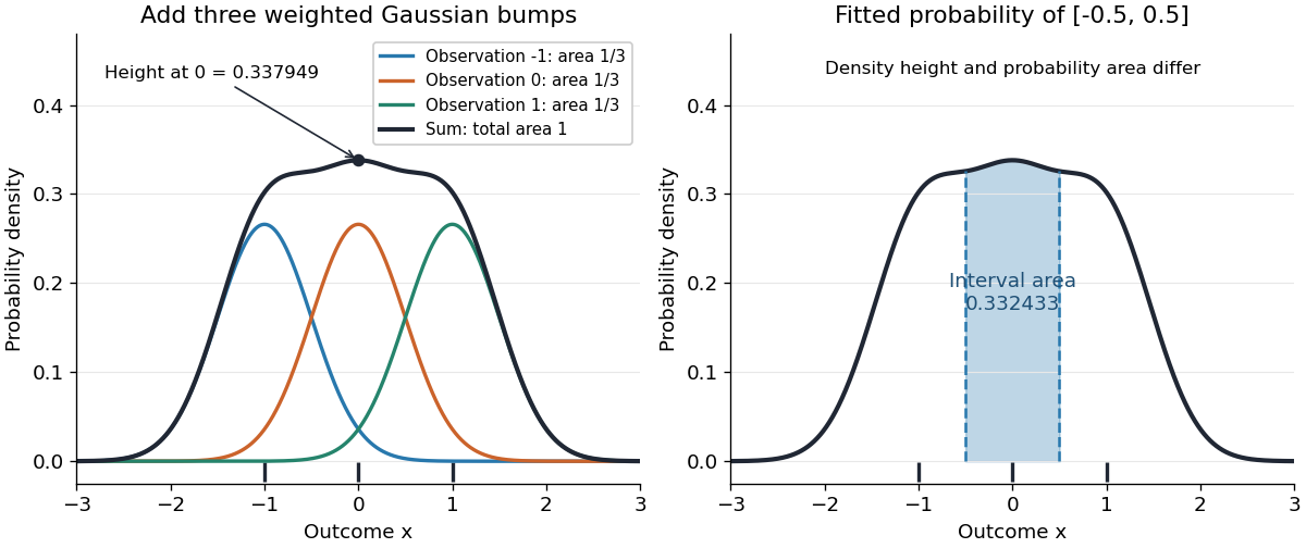
Before the statistical sample is observed, ${\hat{f}}_{n,h,K}$ is a random function; afterwards it is a fitted probability density function. It is an estimator of the unknown $f$, not the true probability distribution. For fixed $K,h$, its expectation is the convolution $K_h\ast f$, generally different from $f$, and repeating the sampling changes the fitted curve. The exact mean integrated squared error of a kernel density estimator separates this smoothing bias of an estimator from sampling variance. Allowing signed kernels of order ell retains the formula but can lose nonnegativity.

A U-statistic kernel is an integrable function of a fixed number r of observations whose expectation is the parameter functional to be estimated. Exchangeability permits symmetrization without changing that expectation. This is a function of r sample values, rather than the one-displacement kernel for density estimation.

For normalized Legendre polynomials, this kernel for density estimation reproduces evaluation at zero on every polynomial of degree below $\ell$: expand $p$ in the orthonormal basis to obtain $\int K_{\ell }p=p(0)$. Taking monomials proves integral one and zero moments of orders $1,\dots ,\ell -1$; compact support gives finite absolute moments. If exact order requires a nonzero moment of order $\ell$, add $({\varphi }_{\ell }(0)+1){\varphi }_{\ell }{1}_{[-1,1]}$. Lower moments remain unchanged. Writing $a_{\ell }=⟨u^{\ell },{\varphi }_{\ell }⟩\ne 0$ and evaluating the full expansion of $u^{\ell }$ at zero shows that the new moment is $a_{\ell }$. A useful three-derivative example is $K_3=(9-15u^2)1_{[-1,1]}/8$, whose first two moments vanish and whose squared L2 norm is $9/8$.

Nonparametric statistics studies statistical inference without restricting the unknown probability distribution or target function to a fixed finite-dimensional parametric statistical model. In density estimation and nonparametric regression, the number of features that an estimator can represent may grow with the sample size. Rank tests offer another approach: the probability distribution of their test statistic under the null hypothesis can be obtained without specifying the common continuous probability distribution.

"Nonparametric" does not mean free of assumptions or tuning choices. A kernel density estimator still requires a kernel for density estimation and a smoothing bandwidth, and its interpretation depends on assumptions about the statistical sample. The freedom is useful when a prescribed shape, such as a single normal distribution, would hide features that the observations might reveal.

Fix the second moment $v>0$. Put $B=\sqrt{5v}$ and $E(u)=3(B^2-u^2{)}_{+}/(4B^3)$. For every nonnegative unit-integral kernel for density estimation $K$ with the same second moment and finite $R(K)$, the mass and second-moment constraints give $\int (B^2-u^2)(K-E)=0$. Outside $[-B,B]$, $E=0$ and $(B^2-u^2)K\le 0$, so $\int E(K-E)\ge 0$. Expanding the square gives $R(K)-R(E)=\int (K-E{)}^2+2\int E(K-E)\ge 0$, with equality only when $K=E$ almost everywhere. Since $R(K{)}^2{\mu }_2(K)$ is scale invariant, rescaled Epanechnikov kernels minimize the optimized asymptotic mean integrated squared error over all such second moments. This conclusion concerns nonnegative second-order kernels; signed higher-order kernels obey a different bias expansion.

A kernel for density estimation is an integrable function K of unit integral, ordinarily nonnegative and centered. Square integrability is needed for integrated variance; a symmetric second-order kernel for density estimation also has $\int uK(u)du=0$ and finite nonzero second moment ${\mu }_2(K)$. Its scaled form is $K_h(u)=h^{-1}K(u/h)$, and the kernel density estimator isHigher-order signed kernels are possible, but need not give a nonnegative probability density function estimate.

The mean integrated squared error is $\mathbb{E}\int ({\hat{f}}_h(x)-f(x){)}^{2}dx$. Put $g_h=K_h\ast f$. Independence gives the pointwise mean $g_h$ and variance $n^{-1}[(K_h^2\ast f)-g_h^2]$. Integrating, use $\int f=1$ and Fubini to obtain $\int (K_h^2\ast f)=R(K_h)$. The bias-variance decomposition proves the exact formulaEquivalently this is $R(f)-2\int f(K_h\ast f)+(1-n^{-1})R(K_h\ast f)+R(K)/(nh)$. These identities assume the displayed integrals are finite; they are exact, rather than a small-smoothing bandwidth expansion.

For a symmetric second-order kernel for density estimation, Taylor expansion gives leading bias $h^2{\mu }_2(K)f^{\prime \prime }/2$, and the leading integrated variance is $R(K)/(nh)$. Thus the asymptotic mean integrated squared error balances inverse smoothing bandwidth against fourth-power bias, with optimal smoothing bandwidth $[R(K)/(n{\mu }_2(K{)}^{2}R(f^{\prime \prime })){]}^{1/5}$. Its appearance of the integrated squared density curvature motivates the scale comparison.

For $f_a(x)=af(ax)$, $a>0$, two differentiations give $f_a^{\prime \prime }(x)=a^3{f}^{\prime \prime }(ax)$. A change of variables therefore gives $R(f_a^{\prime \prime })=a^{5}R(f^{\prime \prime })$, which tends to zero as $a\downarrow 0$ if the original curvature integral is finite. The distribution with probability density function $f_a$ is that of X divided by a, so $\sigma (f_a)=\sigma (f)/a$. ConsequentlyThis scale-invariant density curvature measures shape without dependence on the units used to measure X.

For the final minimization, write $c=35/32$ and use the triweight kernel $f_0=c(1-x^2{)}^3$ on $(-1,1)$, zero outside. Integration gives total mass one, mean zero and variance $1/9$. Its value and its first two derivatives vanish at both endpoints, so its extension is twice continuously differentiable. On the interior,In particular $f_0^{\prime \prime \prime }(1)=-48c$ and $f_0^{\prime \prime \prime }(-1)=48c$.

Put $e=h-f_0$. The mass and moment constraints give $\int e=\int x^{2}e=0$, since both means vanish and their variances match. If $R(h^{\prime \prime })=\infty$ the claim is immediate; otherwise expand the squared norm and integrate its cross term twice by parts over $[-1,1]$. The first endpoint term vanishes because $f_0^{\prime \prime }(\pm 1)=0$, but the next one must be retained:For the second equality use the zero mass and second moment of e and $e=h\ge 0$ outside the support. All terms in the last expression are nonnegative, including the endpoint values of a probability density function. It follows thatThis proves that the triweight density minimizes integrated squared curvature under the specified constraints. Equality forces $e^{\prime \prime }=0$; a globally affine integrable difference of probability density functions is zero, so equality occurs only at $h=f_0$.

Assume a symmetric second-order probability density function kernel for density estimation and enough smoothness for the displayed derivative functionals. The benchmark smoothing bandwidth is $h_0=[R(K)/(n{\mu }_2(K{)}^{2}R(f^{\prime \prime })){]}^{1/5}$, balancing $R(K)/(nh)$ against $h^4{\mu }_2(K{)}^{2}R(f^{\prime \prime })/4$. Three widely used selection methods are as follows.

For least-squares density cross-validation, expand integrated squared error as $R({\hat{f}}_h)-2\int {\hat{f}}_{h}f+R(f)$. Estimate the middle integral by leaving out the observation at which the estimate is evaluated, and minimizeThe left-out observation is independent of its estimator, so the second term has expectation $-2\int (K_h\ast f)f$. Thus $\mathbb{E}\mathrm{CV}(h)=\mathrm{MISE}(h)-R(f)$ exactly. The subtraction of the self-contribution is essential. Computation uses $R({\hat{f}}_h)=n^{-2}{\sum }_{i,j}(K_h\ast {\tilde{K}}_h)(X_i-X_j)$, where ${\tilde{K}}_h(u)=K_h(-u)$. This method directly targets integrated error without estimating a curvature functional first. Under standard smoothness and a suitable search interval its selected smoothing bandwidth is ratio-consistent with the MISE optimum, and hence with $h_0$. Relative fluctuations are ordinarily $O_p(n^{-1/10})$, so the selected values can be quite variable in finite samples.

For biased density cross-validation, estimate curvature from the second-derivative probability density function estimator and subtract its diagonal variance term:Differentiating the kernel for density estimation estimator and applying the integrated-variance identity gives the exact expectation $\mathbb{E}R({\hat{f}}_h^{\prime \prime })=R(K^{\prime \prime })/(n{h}^5)+(1-n^{-1})R(K_h\ast f^{\prime \prime })$. Under the derivative regularity assumptions, $R(K_h\ast f^{\prime \prime })=R(f^{\prime \prime })+O(h^2)$, so $\mathbb{E}{\hat{A}}_h=R(f^{\prime \prime })+O(h^2)+O(n^{-1})$. Minimize BCV over a reasonable smoothing bandwidth range. It is a smoothed criterion directed at AMISE; the name reflects its finite-sample bias rather than an exact unbiased-risk identity. Standard conditions again give ratio consistency and relative fluctuation order $n^{-1/10}$. It often has a smoother objective than ordinary least-squares cross-validation, though numerical behavior and relative variance depend on the probability density function and kernel for density estimation.

For plug-in bandwidth selection, obtain an independent pilot scale g, estimate $A=R(f^{\prime \prime })$, then setThe pilot should be positive and stable; consistent positive estimates make this expression ratio-consistent by continuity. A simple normal-reference initialization uses $R(f^{\prime \prime })=3/(8\sqrt{\pi }{\sigma }^5)$ under a normal reference model, substituting a sample scale for sigma. For a Gaussian density kernel this gives $h\approx 1.06\hat{\sigma }{n}^{-1/5}$. A pure normal-reference rule is quick but is asymptotically correctly calibrated only when its assumed curvature matches the actual probability density function; it is useful as the first stage of a data-driven plug-in procedure.

A more adaptive fourth-derivative pilot estimate of density curvature uses $R(f^{\prime \prime })=\int f{f}^{(4)}$, obtained by two integrations by parts, and estimates it byThe diagonal expectation contributes $K^{(4)}(0)/(n{g}^5)$; the leading smoothing bias is $-g^2{\mu }_2(K)R(f^{\prime \prime \prime })/2$. Balancing these terms produces the stated pilot scale $g\asymp R(f^{\prime \prime \prime }{)}^{-1/7}{n}^{-1/7}$, with another pilot or reference model supplying $R(f^{\prime \prime \prime })$. Under sufficient derivatives and tail control, its error is bounded byat that pilot scale. Taylor expansion of the fifth-root formula gives ${\hat{h}}_{\mathrm{PI}}/h_0-1=-(\hat{A}-A)/(5A)+o_p(|\hat{A}-A|)$, so it inherits that bound. A calibrated cancellation of leading pilot bias can give a faster rate. This illustrates why an appropriately constructed plug-in selector can converge more quickly than cross-validation, while requiring more smoothness and pilot choices. For each ratio-consistent method, its attained AMISE divided by the minimal AMISE tends to one.

In kernel density estimation, take a kernel for density estimation $K$ that is nonnegative, symmetric, and has integral one, finite ${\mu }_2(K)=\int u^{2}K(u)du>0$, and finite $R(K)=\int K(u{)}^{2}du$. Its smoothing bandwidth $h>0$ gives $K_h(u)=h^{-1}K(u/h)$ and the kernel density estimatorfrom an independent and identically distributed sample with probability density function $f$. Nonnegativity and unit mass make the estimate itself a probability density function. We compare kernel for density estimation shapes by their optimized mean integrated squared error, rather than by their performance at an arbitrarily common numerical smoothing bandwidth.

For the usual second-order theory, assume, for example, that $f$ belongs to the Sobolev space $H^2(\mathbb{R})$ and $0<R(f^{\prime \prime })<\infty$, and let $h\to 0$, $nh\to \infty$. The expectation is the convolution $K_h\ast f$. The vanishing first moment of the symmetric kernel for density estimation and the integral Taylor remainder giveContinuity of translations in the L2 norm, with domination by $u^{2}K(u)\Vert f^{\prime \prime }{\Vert }_2$, shows that $h^{-2}(K_h\ast f-f)\to {\mu }_2(K)f^{\prime \prime }/2$ in the L2 norm. Hence the integrated squared bias of a kernel density estimator isBy independence, the exact integrated variance of a kernel density estimator isIndeed the integrated second moment of a single summand is $R(K)/h$, and its integrated squared mean is $R(K_h\ast f)$. The latter quantity is bounded by $R(f)$, by Young's convolution inequality, so its contribution is $O(n^{-1})$. The bias-variance decomposition of mean squared error therefore yields the leading criterionThis asymptotic mean integrated squared error displays the bias-variance tradeoff: a small smoothing bandwidth increases integrated variance, while a large one increases squared bias of an estimator.

Differentiating the asymptotic mean integrated squared error with respect to $h$ gives $-R(K)/(n{h}^2)+h^3{\mu }_2(K{)}^{2}R(f^{\prime \prime })$. It changes sign once, from negative to positive, so its unique minimum isAt this minimum the integrated variance term is four times the squared bias of an estimator term. Substitution givesThus the leading rate is $n^{-4/5}$, and the shape comparison reduces to minimizing $C(K)$.

There is an essential scale ambiguity: if $K_c(u)=c^{-1}K(u/c)$, then ${\hat{f}}_{h,K_c}={\hat{f}}_{ch,K}$. Changing the scale of the kernel for density estimation merely changes the numerical convention for the smoothing bandwidth. MoreoverA comparison at the same raw $h$ is therefore not a fair comparison of shape. One can normalize the second moment to one, but that does not make the optimal smoothing bandwidth independent of shape.

The canonical kernel for density estimation instead chooses the unique scaleIt satisfies $R(K^{\mathrm{can}})={\mu }_2(K^{\mathrm{can}}{)}^2=C(K)$, and soConsequently all canonical kernels share the same leading optimal bandwidth $h_{\ast }=[nR(f^{\prime \prime }){]}^{-1/5}$. Only the multiplicative constant $C(K)$ depends on shape. This is precisely the separation of shape choice and scale choice that makes the canonical kernel normalization useful. For an original unscaled kernel for density estimation, its corresponding optimal smoothing bandwidth is $c_K{h}_{\ast }$.

To prove optimal shape, scale a candidate kernel for density estimation to have second moment one. Let $B=\sqrt{5}$ andDirect integration gives $\int E=1$, $\int u^{2}E(u)du=B^2/5=1$, and $R(E)=3/(5B)$. Thus $E$ is a rescaled Epanechnikov kernel. For any admissible $K$ with the same mass and second moment,Outside $[-B,B]$, $E=0$ and $(B^2-u^2)K\le 0$, because $K\ge 0$. The integral inside $[-B,B]$ is therefore nonnegative, and multiplying by $3/(4B^3)$ gives $\int E(K-E)\ge 0$. Expanding the square now provesEquality forces $K=E$ almost everywhere. At fixed second moment, minimizing $R(K)$ is equivalent to minimizing $C(K)$. Since $C(K)$ is scale invariant, this proves the optimality of the Epanechnikov kernel over all nonnegative symmetric second-order kernels for density estimation, including the equality case up to rescaling.

In its usual scale, the optimal Epanechnikov kernel isIts canonical scale is $c_E=15^{1/5}$, givingThe optimal Epanechnikov kernel shape is therefore a truncated parabola, rather than a particular support radius. The canonical kernel and unit-second-moment version represent the same shape but different scale conventions.

The numerical gains over other reasonable kernels for density estimation are modest. Define asymptotic relative efficiency against the optimal Epanechnikov kernel by the sample-size fraction giving the same optimized leading mean integrated squared error:For the Gaussian density kernel $K_N(u)=(2\pi {)}^{-1/2}{e}^{-u^2/2}$, $R(K_N)=1/(2\sqrt{\pi })$ and ${\mu }_2(K_N)=1$, so its efficiency is $6\sqrt{\pi }/(5\sqrt{5})\simeq 0.9512$. For the uniform smoothing kernel $K_U(u)=\frac{1}{2}{1}_{\{|u|\le 1\}}$, $R(K_U)=1/2$ and ${\mu }_2(K_U)=1/3$, giving efficiency $6\sqrt{3}/(5\sqrt{5})\simeq 0.9295$. The Gaussian density kernel is infinitely smooth, whereas the optimal Epanechnikov kernel has compact support and allows each observation to affect only a finite window. Such computational and smoothness considerations may outweigh a small leading-efficiency difference.

In practice $R(f^{\prime \prime })$ is unknown. A plug-in estimator estimates this roughness functional from a pilot estimate of the second derivative and substitutes it into the optimal smoothing bandwidth formula. Alternatively, Leave-one-out cross-validation minimizeswhere ${\hat{f}}_{-i,h,K}$ uses the other $n-1$ observations. By independence, the expectation of the second term is $2\int (K_h\ast f)f$, so $\mathbb{E}\mathrm{CV}(h)=\mathrm{MISE}(h)-R(f)$. Thus it targets integrated error without knowing $f$. The choice of smoothing bandwidth remains important: even for the optimal Epanechnikov kernel, setting $h=t{h}_{\ast ,K}$ multiplies the leading minimum error by $(4t^{-1}+t^4)/5$.

The preceding optimum concerns nonnegative second-order kernels for density estimation and twice-smooth densities on the real line. Signed kernels of order ell can cancel higher moments for smoother densities and yield different rates, but may produce negative density estimates. A support boundary or a density jump also requires separate bias of a kernel density estimator analysis. These settings do not contradict the proved second-order optimality of the Epanechnikov kernel.