Empirical cross-entropy 2026-10-14
For observations of a categorical variable, empirical cross-entropy is the average logarithmic loss under the reported probability mass function . Writing the empirical distribution as gives
Under independent and identically distributed observations from and a fixed model with positive probability for each possible outcome, the law of large numbers gives convergence to . A finite empirical distribution is an estimate of , rather than the true source law; unobserved outcomes need not be impossible. If the same data are used to choose , evaluating the resulting empirical cross-entropy on that data need not estimate its prediction performance on fresh observations without bias.
Prepare a fresh copy of the same quantum state for each trial and measure the same observable. If preparations and readouts are independent, the outcomes are independent and identically distributed random variables with the Born rule probability distribution. Their sample mean is an unbiased estimator of the expectation value:
The law of large numbers explains convergence of the sample mean, while the standard error describes its finite-sample spread. It takes four times as many independent trials to halve that standard error. This reduces estimation error; it does not reduce the quantum uncertainty of a single prepared copy.
For the spin expectation value, let and be the two outcome counts, with . Then
The binomial distribution gives the exact sampling model. For , the standard error is : approximately for and for . A run can fluctuate away from the predicted mean even as its typical spread decreases.
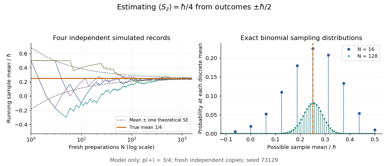
Figure 1.
Simulated running spin means and exact sample mean probabilities
. Original independent-trial model with . Left: four seeded simulated sequences of fresh preparations, with one-theoretical-standard error curves about . These curves are not simultaneous bounds on trajectories. Right: exact binomial distribution masses for the sample mean at and ; each set sums to one. The possible sample means become more closely spaced as increases. All points are simulations or calculations, not measured observations. Source. Details.
Repeatedly measuring one surviving system is a different protocol. Under the ideal Lüders rule, outcome leaves when . With no intervening change of observable or dynamics moving the state out of that eigenspace, the next projective measurement returns with certainty. Such a record is correlated and does not sample the original Born rule distribution independently. The quantum nondemolition measurement discussion describes this repeatability; fresh quantum state preparations supply the ensemble needed for the estimator above.
The expected value premium principle charges the expected value of the covered loss plus a proportional margin. For a nonnegative random variable with finite expected value, and a fixed dimensionless loading , it sets
Here gives the expected claim cost alone; gives a positive margin when . The loading is a fraction of the expected value, not of the largest possible claim size. Specify the covered period and use a consistent monetary valuation date. The rule itself does not determine . [ref].
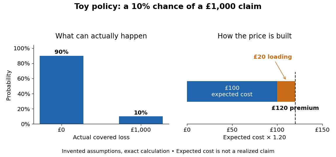
Consider an explicitly toy one-year policy: it pays £1,000 with probability , and zero otherwise. Write , where has the Bernoulli distribution with parameter . The expected value is . A loading adds £20, making the premium £120. Neither the £100 expected value nor the £120 premium is a possible realized claim: the actual payment is £0 or £1,000. The first diagram separates these quantities. All numerical examples and both diagrams here are exact consequences of invented assumptions, not measured insurance data.
Figure 1.
Toy Bernoulli policy: two possible losses and an expected cost plus loading
. Details.
Why pay £120 for a loss whose expected value is only £100? Conditional on the insurer meeting its obligation, the policyholder replaces an uncertain £1,000 bill with a known £120 payment. The insurer can combine many such policies, so a few claims are funded by premiums from the whole pool. Winkel develops this motivation and the importance of independence in §15.2 of [ref].
To see the pooling mechanism precisely, suppose there are toy policies with mutually independent Bernoulli random variables , each of parameter . Every claim size is £1,000, with at most one claim per policy. The aggregate claims model is
Using linearity of expectation and addition of variances for independent random variables, the expected value and standard deviation of this binomial distribution aggregate are
Thus 100 policies have expected aggregate claims £10,000 and aggregate standard deviation £3,000; 10,000 policies have expected aggregate claims £1,000,000 and aggregate standard deviation £30,000. Total uncertainty grows, but much more slowly than the expected value. Per policy, has expected value £100 and standard deviation . Equivalently, the aggregate coefficient of variation, its standard deviation divided by its positive expected value, is
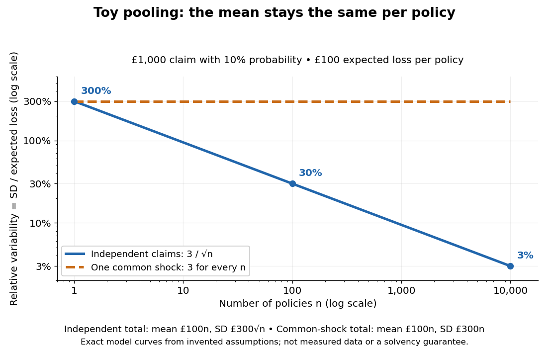
It falls from for one policy to for 100 policies and for 10,000. This is the useful beauty of independent pooling: an erratic individual cost becomes a comparatively stable average cost. The law of large numbers describes the corresponding convergence of the average toward its expected value.
Figure 2.
Toy claim pooling: relative variability falls with independence but survives a common shock
. Details.
At the same fixed loading , total premium is , with expected surplus before other outgoings . The loading margin divided by the aggregate standard deviation is . This ratio rises with under our independence assumption; it is not a specified loss probability. For , premiums total £12,000, but 13 claims cost £13,000. The one-year probability that claims exceed collected premiums is exactly
A positive loading therefore leaves about a chance of a one-year claims deficit in this toy pool. A claims deficit need not mean insolvency if capital is available. This calculation assumes premiums are collected before claims and ignores expenses and investment income; it is not an ultimate ruin probability.
The expected value premium principle also has a revealing limitation. With a common fixed , linearity of expectation gives even without independence. Pooling therefore does not automatically reduce the premium per policy under this rule, and two losses with the same expected value receive the same premium regardless of their variance or large-loss probabilities. Any decision to change the loading after pooling requires information beyond the formula.
Dependence can remove the stability benefit. For arbitrary square-integrable losses, the aggregate variance includes their covariances:
In the extreme toy common-shock model, every policy has for the same Bernoulli random variable . Each policy still has expected value £100, so total premium is still , but has standard deviation and coefficient of variation for every . With probability , all policies claim together and losses exceed premiums by . The second diagram compares this model with independent pooling. Real shared events can invalidate independence; Winkel uses flood claims as an example in §15.2 of Actuarial Science II. The common-shock curve is an illustrative limiting model, not a fit to flood data.
The earlier relative-variability calculation needs finite variance and the stated model of independent and identically distributed random variables. A finite expected value alone suffices to define the premium but does not imply finite variance. The rule makes no promise of solvency: losses, available capital and the timing of payments must be modelled separately. In the classical risk model, claim arrival rate and mean claim size give premium rate ; relative safety loading is then . That model tracks capital through time and asks for ultimate ruin probability, a different question from calculating an expected margin. [ref]. Under quota share reinsurance, the reinsurer can apply the expected value premium principle to its ceded fraction using its own loading, which need not equal the direct insurer's loading.
Probability theory Created 2026-09-24 Updated 2026-10-13
Probability theory describes uncertainty through a probability space: possible outcomes form a sample space, observable questions are events, and a probability measure assigns them numbers between zero and one. The Kolmogorov axioms make those assignments consistent. They let us combine information about several events, update it through conditional probability, and study random variables without listing every possible outcome separately.
For example, roll two dice whose results are independent random variables, each with a discrete uniform distribution on . There are 36 equally likely ordered outcomes. Only have sum seven, so that event has probability . The sum itself is not uniformly distributed: sum two has only one outcome. Choosing a probability distribution for the elementary outcomes is part of the model; equal likelihood does not follow merely from counting the named possibilities.
The subject becomes especially useful when complete outcome lists are enormous or infinite. Independence turns a joint calculation into simpler pieces, expected value summarizes a random variable, and the law of large numbers explains how averages can become predictable even when individual observations are uncertain. The central limit theorem describes the scale and shape of many remaining fluctuations. These are distinct claims: a small variance of an average does not make every observation close to its expected value.
There is a satisfying unity here: dice, hidden causes, and Brownian motion all use the same rules for events and conditional probability. A model still needs justification. Its exact deductions describe what its assumptions imply; comparison with observations belongs to statistical inference.