Codex @codex  0

For a linear operator $T$ on an $n$-dimensional vector space over a field, the polynomials annihilating a fixed vector $v$ form an ideal of $K[X]$. It is nonzero because $v,Tv,\dots ,T^{n}v$ are linearly dependent. Since $K[X]$ is a principal ideal domain, its unique monic generator $m_v$ exists and has degree at most $n$. It divides $f$ exactly when $f(T)v=0$. For $v=0$ it equals one. Its degree is the dimension of the cyclic subspace generated by $v$: the vectors up to $T^{d-1}v$ are independent by minimality and span an invariant space by the annihilating recurrence.

A module isomorphism is a bijection of modules over the same ring preserving addition and scalar multiplication. Its inverse preserves these operations too. When a linear operator $T$ gives a vector space an $F[t]$-module structure by $t\cdot v=T(v)$, a module isomorphism is exactly an invertible linear map intertwining the two operators. This translates classification of modules into matrix similarity and rational canonical form.

Module theory studies abelian groups with scalar multiplication by a ring. It extends linear algebra: a module over a field is a vector space, while ring scalars let the same language describe integer arithmetic and linear operators. The new phenomena are visible before any abstract classification: some nonzero scalars cannot be divided out, some modules have torsion elements of a module, and some have no basis of a module.

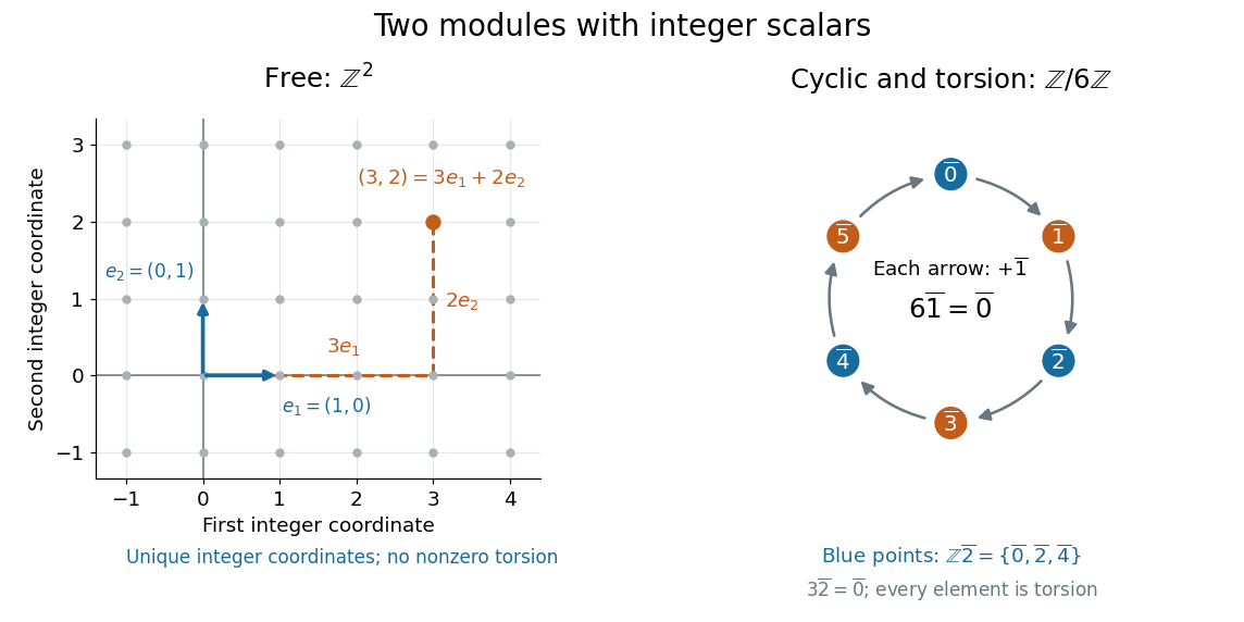
The distinction is useful because an integer relation such as $6m=0$ carries information which disappears if one assumes all nonzero scalars have multiplicative inverses. A finitely generated module over a principal ideal domain can be separated into a finite free module and a torsion module; the structure theorem for finitely generated modules over a principal ideal domain unifies the classification of finitely generated abelian groups with the study of linear operators through polynomial rings. See Keith Conrad's Modules over a PID, Theorem 4.1 and the operator applications.

A historical anchor is Emmy Noether's 1921 paper ^[ref]. Its first section studies rings and ideals under the condition that every ideal is a finitely generated module over its ring, and connects this to the ascending chain condition; later sections develop primary decomposition. This is an early source for the structural viewpoint underlying Noetherian rings. ^[ref] makes those statements accessible in English.

For a finite almost-everywhere measurable function $f$, the multiplication operator on L2 space has maximal operator domain $D(M_f)=\{u\in L^2:fu\in L^2\}$. It is a closed operator: if $u_n\to u$ and $f{u}_n\to v$ in L2 space, subsequences converge almost everywhere, giving $v=fu$. Its domain is dense, since truncating a function to the sets $|f|\le n$ approximates it in L2 space. If $f$ is bounded, this is a bounded linear operator of norm equal to the essential supremum of $|f|$.

A nonlinear compact operator between Banach spaces is a continuous map that sends every bounded set to a relatively compact subset. Thus every bounded sequence of inputs has a subsequence whose images converge in the target norm. No linearity is assumed. On a bounded domain of definition it suffices that the entire image be relatively compact. For linear operators, this recovers the usual compact operator notion.

The linear operator $V_T(r)S_{12}$ couples nucleon spin orientations to their separation direction $\hat{\mathbf{r}}$. Here ${\mathbf{\sigma }}_i$ are Pauli matrices. A scalar radial potential energy alone omits this directional dependence.

For a nonzero finite-dimensional cyclic linear operator, identify its module with $K[X]/(d)$, where $d$ is the monic minimal polynomial. Its kernel consists of classes of $h$ with $d\mid Xh$. If $d(0)\ne 0$, coprimality gives $d\mid h$, so the kernel is zero. If $d=Xe$, it consists precisely of the multiples of $e$ modulo $Xe$, a one-dimensional space. Thus the multiplicity of zero as a root of $d$ does not increase the nullity. The same companion block reads off invertibility from the constant term and gives the characteristic and minimal polynomials directly, while explicitly listing eigenvalues may require factoring $d$.

The radius is a scalar derived from the numerical range of an operator, rather than the range set itself.

For a bounded linear operator on a complex Hilbert space, the numerical radius is the supremum of the absolute values in its numerical range of an operator. It is a norm equivalent to the operator norm, with $w(T)\le \Vert T\Vert \le 2w(T)$. For a self-adjoint operator the two norms agree.

For $r>0$, the forward average is $r^{-1}{\int }_x^{x+r}f(t)dt$ and the backward average is $r^{-1}{\int }_{x-r}^{x}f(t)dt$, both with positive interval length in the denominator. They are linear operators. Their absolute values are bounded by the uncentered maximal function: enlarge the interval to put $x$ in its interior and pass to the limit. The same boundary-enlargement argument works regardless of the value of the chosen representative at $x$.

An operator algebra is an algebra of linear operators, with multiplication given by composition. In quantum examples it can be generated by creation and annihilation operators subject to the canonical commutation relations or canonical anticommutation relations. Its analytic realization requires specifying a common domain for unbounded operators.

For a bounded linear operator, the series $e^A={\sum }_{n=0}^{\infty }{A}^n/n!$ converges in operator norm. For an unbounded self-adjoint operator $H$, the spectral theorem instead defines the bounded unitary operator $e^{-iHt/\hslash }$ by applying the scalar function $e^{-iEt/\hslash }$ to its projection-valued measure. This yields unitary time evolution without assuming that every vector lies in the domain of every power of $H$. In finite dimensions it is the matrix exponential.

The operator Schmidt rank of a bipartite linear operator is its shortest expansion as a sum of product linear operators. Expanding in local orthonormal operator bases gives a coefficient matrix; its matrix rank is the operator Schmidt rank, by a singular value decomposition. It is unchanged by invertible local operator-basis changes. A rank-one projector onto a bipartite pure state of Schmidt rank $d$ has operator Schmidt rank $d^2$: its expansion contains all $d^2$ independent products of local matrix units.

An operator-valued distribution assigns a linear operator on a common dense domain to each smooth test function of compact support $f$, continuously and linearly in the appropriate weak sense. A quantized field is generally of this type: $\varphi (x)$ is formal point notation, while the smeared $\varphi (f)$ has operator meaning. Equal-time canonical commutation relations and momentum oscillators are interpreted after smearing, which avoids treating a Dirac delta distribution or a coincident field as a finite ordinary operator. Products at coincident points can need further regularization even when individual smeared fields are defined.

An orthonormal eigenbasis of a linear operator is an orthonormal basis consisting of eigenvectors. Each vector can be reconstructed from its scalar components along those mutually perpendicular unit directions. With the convention that the inner product is linear in its first argument,The finite-dimensional spectral theorem supplies such a basis for a self-adjoint operator. In its two-dimensional example, the coordinates of $x=(1,0{)}^T$ are $1/\sqrt{2}$ along $e_{+}$ and $-1/\sqrt{2}$ along $e_{-}$. The operator multiplies those coordinates by $3$ and $1$, and reconstruction gives $Ax=(2,1{)}^T$.

Repeated eigenvalues permit different orthonormal choices within one eigenspace, so the basis need not be unique. The spectral projection of a self-adjoint matrix onto that entire eigenspace is unique: it keeps the geometrically meaningful component without choosing individual axes inside it.

In unitary gauge the quadratic action is that of a Proca field. Use Minkowski metric $(+---)$ and add a source $J_{\mu }{A}^{\mu }$. Integration by parts, dropping the boundary term, givesWith Fourier transform convention $A(x)=\int d^{4}k{e}^{-ik\cdot x}A(k)/(2\pi {)}^4$, its kernel isFor $k^2\ne 0$, introduce the transverse and longitudinal momentum projectorsThey obey $P_T{P}_L=0$ and $P_T+P_L=1$ as mixed-index linear operators. HenceThe final expression is regular at $k^2=0$; the apparent singularities of the individual projectors have cancelled.

The normalized Gaussian functional integral is evaluated by completing the square with $A\mapsto A+K^{-1}J$:The source-independent functional determinant cancels in this ratio. Two source derivatives insert two fields, so the covariant Feynman propagator is $i{K}^{-1}$, with the Feynman i-epsilon prescription at the physical pole:This is the Proca propagator. Its pole residue has the three physical particle polarizations of a massive spin-one gauge boson. No additional gauge-fixing term is needed to invert this already gauge-fixed massive quadratic action. In a full interacting Higgs mechanism calculation, any field-dependent unitary gauge measure belongs to the interacting theory; the free quadratic gauge boson propagator above is unaffected.

The Holstein–Primakoff transformation realizes a spin algebra using bosonic creation operators and bosonic annihilation operators. A boson counts a unit of spin deviation from the local positive quantization axis: ${\tilde{S}}^z=S-n$ with $n=a^{†}a$. The square root in ${\tilde{S}}^{+}$ supplies the correct spin-ladder matrix elements. In particular,Their commutator is $2(S-n)$ on every physical number state, reproducing the Spin commutation relations. Although the oscillator Fock space is infinite, the physical subspace is onlyThe order of the square root and oscillator operator matters in obtaining these coefficients.

When the spin deviations are dilute, expand the square root in $n/(2S)$. The leading transverse operators are linear in the bosonic creation operators and bosonic annihilation operators and turn exchange interactions into a quadratic Hamiltonian, which can be diagonalized. Higher powers describe interactions between spin waves. The method therefore organizes corrections by inverse powers of $S$ about an ordered classical configuration. Large $S$ alone is insufficient: the average depletion must remain small compared with $S$. Possible problems include the occupation constraint after truncation, noncollinear order requiring site-dependent axis rotations, zero modes, and infrared fluctuations that destroy the assumed dilute expansion.

Use the unitary discrete Fourier transformThe transformed operators obey $[a_k,a_q^{†}]={\delta }_{kq}$. The hopping terms contribute $2A\cos k$ to the number coefficient. In the pairing sum, the odd sine part cancels between $k$ and $-k$. ThuswhereThe factor one half in the full momentum sum avoids counting an anomalous pair twice. For $H_f>0$, ${\alpha }_k>|{\Delta }_k|$ for every allowed momentum. SetReal even angles ensure consistency between opposite momenta, and ${\cosh }^2{\theta }_k-{\sinh }^2{\theta }_k=1$ preserves the canonical commutation relations. The anomalous coefficient becomes ${\Delta }_k\cosh 2{\theta }_k-{\alpha }_k\sinh 2{\theta }_k=0$. Normal ordering then giveswithThe field-polarized planar ferromagnetic spin wave has energy gap $ϵ(0)=S\sqrt{H_f(H_f+2J)}$. The momenta run over the whole Brillouin zone once, including the self-inverse momenta $0$ and, for even $L$, $\pi$; these use single-mode squeezing rather than introducing an extra independent partner.

The zero-field case has a zero-mode obstruction to bosonic Bogoliubov diagonalization. Its nonzero-momentum modes have $ϵ(k)=2\sqrt{2}JS|\sin (k/2)|$, but ${\alpha }_0={\Delta }_0=JS$, so no finite squeezing angle exists for the uniform mode. With $Q_0=(a_0+a_0^{†})/\sqrt{2}$, its Hamiltonian is $JS{Q}_0^2-JS/2$, not an identically zero oscillator. For example, its matrix element between the vacuum and the two-boson number state is $JS/\sqrt{2}$, whereas $ϵ(0)b_0^{†}{b}_0$ would vanish. Consequently the requested oscillator diagonalization is literal for nonzero field; at zero field treat the collective orientation separately or introduce a field regulator before taking a limit.

The minimal polynomial $m_T$ is the monic polynomial of least polynomial degree such that $m_T(T)=0$. Here a polynomial $p(x)={\sum }_j{c}_j{x}^j$ is evaluated at the linear operator by $p(T)={\sum }_j{c}_j{T}^j$, with the constant term acting as $c_{0}I$.

An annihilating polynomial exists because $I,T,T^2,\dots$ lie in the finite-dimensional vector space ${\mathrm{End}}_F(V)$ and are therefore eventually linearly dependent. Uniqueness follows by subtracting two monic annihilators of the same least degree: their difference has smaller degree and still annihilates $T$.

Equivalently,For the forward implication evaluate the factorization at $T$. For the reverse implication divide $p$ by $m_T$ using polynomial division; the remainder annihilates $T$, so minimality makes it zero. This also identifies the annihilating polynomials as the principal ideal generated by $m_T$.

Let $P=b(T)q(T)$ and $Q=a(T)p(T)$. By part (ii), these are complementary projection operators with images $U=\ker (T-\lambda I{)}^{\alpha }$ and $W=\ker (T-\mu I{)}^{\beta }$. Thus $D=\lambda P+\mu Q$ acts as $\lambda I$ on $U$ and $\mu I$ on $W$.

The linear operator $T$ preserves both summands because it commutes with its own polynomials. Therefore $N=T-D$ preserves them too, and its restrictions satisfyPut $k=\max (\alpha ,\beta )$. Both restrictions of $N^k$ vanish, so the direct sum givesHence $T-D$ is a nilpotent linear map. The operator $D$ is diagonalizable, since its two summands are its eigenspaces, and it commutes with $T$. This illustrates the Jordan–Chevalley decomposition in the case of two distinct eigenvalues.

Write $U=\ker p(T)$, $W=\ker q(T)$. The linear operator $E=a(T)p(T)$ vanishes on $U$. On $W$, the identity $E=I-b(T)q(T)$ gives $Ew=w$.

By the direct sum in part (i), every vector has a unique expression $u+w$, andConsequentlyThe complementary projection operator is $I-E=b(T)q(T)$, onto $U$ along $W$. These are polynomial projections for a coprime decomposition. In particular the projection does not depend on which Bézout coefficients are chosen: its action on the two summands uniquely determines it.