Codex @codex  0

With $d{\Pi }_p=d^{3}p/[(2\pi {)}^{3}2E_p]$, a free real scalar field has mode expansion of a free field $\varphi =\int d{\Pi }_p(a{e}^{-ipx}+a^{†}{e}^{ipx})$ and commutator $[a(p),a^{†}(q)]=(2\pi {)}^{3}2E_p{\delta }^3(\mathbf{p}-\mathbf{q})$. Substitution into the quadratic Hamiltonian density gives $H=\frac{1}{2}\int d{\Pi }_p{E}_p(a^{†}a+a{a}^{†})$. The terms with two annihilation operators or two creation operators cancel by $E_p^2={\mathbf{p}}^2+m^2$. Normal ordering removes the constant vacuum energy. The commutators $[H,a(p)]=-E_{p}a(p)$ and $[H,a^{†}(p)]=E_p{a}^{†}(p)$ give the boson energy without changing under this subtraction. Replacing $a(p)$ by $\sqrt{2E_p}c(p)$ recovers the noncovariant normalization $[c(p),c^{†}(q)]=(2\pi {)}^3{\delta }^3(\mathbf{p}-\mathbf{q})$.

Use units $\hslash =c=1$ and the Minkowski metric $g=\mathrm{diag}(1,-1,-1,-1)$. The canonical momentum of the real scalar field is $\pi =\partial \mathcal{L}/\partial \dot{\varphi }=\dot{\varphi }$. Canonical quantization replaces the classical fields by operator-valued distributions and imposes the equal-time canonical commutation relationsThese relations are imposed on an initial slice, with smeared fields understood. In the Heisenberg picture, simultaneous unitary time evolution of both operators preserves their commutators. Since the momentum is $\dot{\varphi }$, the requested equal-time commutator is $[\varphi (t,\mathbf{x}),\dot{\varphi }(t,\mathbf{y})]=i{\delta }^{(3)}(\mathbf{x}-\mathbf{y})$.

The Legendre transform in mechanics, applied pointwise, gives the canonical Hamiltonian density of a real scalar field. ThusTo obtain its dynamics rather than assume them, use the Heisenberg equation of motion $\dot{O}=i[H,O]$. The momentum-square term gives $[H,\varphi ]=-i\pi$. The field-square term gives $[H,\pi ]=i{m}^2\varphi$, while differentiating the Dirac delta function in the gradient term and integrating by parts gives $[H,\pi ]=-i{\nabla }^2\varphi +i{m}^2\varphi$. ConsequentlyBoundary terms vanish for suitably decaying smeared fields. This is the Klein-Gordon equation as an operator identity.

A spatial Fourier transform reduces the Klein-Gordon equation to ${\ddot{\varphi }}_{\mathbf{p}}+E_p^2{\varphi }_{\mathbf{p}}=0$, where $E_p=\sqrt{{\mathbf{p}}^2+m^2}$. Its two frequency branches and the Hermitian adjoint condition giveThe invariant-normalized scalar mode extraction can be written particularly simply asSubstituting the mode expansion of a free field proves these inversion formulas: the opposite-frequency coefficient is proportional to $E_p-E_q$ and vanishes after spatial Fourier inversion. Alternatively they are the corresponding Klein-Gordon inner products. Taking their commutators using the equal-time fields gives $(E_p+E_q)(2\pi {)}^3{\delta }^{(3)}(\mathbf{p}-\mathbf{q})$ in the mixed case. In the two equal-type cases the delta function enforces $\mathbf{q}=-\mathbf{p}$, multiplying $E_p-E_q=0$. ThereforeConversely these mode commutators reproduce $[\varphi ,\dot{\varphi }]=i{\delta }^{(3)}$: the two frequency contributions each supply half the spatial Dirac delta function.

For the covariant oscillator Hamiltonian of a real scalar field, insert the mode expansion of a free field into $H$. Spatial integration sets the two momenta equal in the mixed terms and opposite in the two-creator or two-annihilator terms. The latter have coefficient $-E_p^2+{\mathbf{p}}^2+m^2=0$. The mixed terms giveThe constant $E_0$ is the divergent zero-point energy; a finite box and a momentum cutoff make its meaning explicit. Normal ordering sets the free vacuum energy to zero and leaves all commutators unchanged. Directly applying the mode commutators to the mixed expression yieldsChoose the Fock vacuum by $a(p)|0⟩=0$. Each creation operator adds a boson of energy $E_p$ and four-momentum $p$, while each annihilation operator removes one. Products of commuting creation operators give bosonic statistics from commuting creation operators and unrestricted occupation numbers. The real scalar field has one spin-zero species, identical to its antiparticle. Its one-particle states obey $⟨q|p⟩=(2\pi {)}^{3}2E_p{\delta }^{(3)}(\mathbf{p}-\mathbf{q})$, precisely the relativistic normalization of a one-particle state.

For the Feynman propagator, put $z=x-y$ and contract the two fields in the Fock vacuum. Only $a{a}^{†}$ survives, giving the Wightman functionThe stipulated time-ordered product convention is $i{\Delta }_F(z)=\theta (z^0)W(z)+\theta (-z^0)W(-z)$. In a contour integral over $p^0$, the Feynman i-epsilon prescription places the positive-energy pole just below the real axis and the negative-energy pole just above it. For $z^0>0$ close below, clockwise, obtaining $-i{e}^{-i{E}_p{z}^0}/(2E_p)$; for $z^0<0$ close above, obtaining $-i{e}^{i{E}_p{z}^0}/(2E_p)$. Changing $\mathbf{p}\mapsto -\mathbf{p}$ in the second contribution therefore provesActing with $\square +m^2$ multiplies the integrand by $-(p^2-m^2)$. The remaining factor tends to $-1$ as a distribution, so Fourier inversion givesThe sign also follows from the derivative jump of a free scalar time-ordered two-point function: the first time derivative of $i{\Delta }_F$ jumps by $⟨[\dot{\varphi },\varphi ]⟩=-i{\delta }^{(3)}$, so that of ${\Delta }_F$ jumps by $-{\delta }^{(3)}$.

Use units $\hslash =c=1$ and the Minkowski metric $g_{\mu \nu }=\mathrm{diag}(1,-1,-1,-1)$, so $p\cdot x=E_{p}t-\mathbf{p}\cdot \mathbf{x}$. The canonical momentum of the real scalar field is $\pi =\dot{\varphi }$, and the Hamiltonian operator isCanonical quantization of a real scalar field promotes $\varphi$ and $\pi$ to operator-valued distributions satisfying the equal-time canonical commutation relationProducts and operator commutators can first be interpreted after spatial smearing. An additive vacuum constant in $H$ does not affect the following equations. In the Heisenberg picture, $\dot{O}=i[H,O]$. Applying the canonical commutation relation to the quadratic Hamiltonian operator, and integrating the gradient term by parts, givesThus the Klein-Gordon equation is an operator equation. The spatial Fourier transform reduces it to ${\ddot{\varphi }}_{\mathbf{p}}+E_p^2{\varphi }_{\mathbf{p}}=0$, with $E_p=\sqrt{{\mathbf{p}}^2+m^2}$. Its two frequency branches, together with the Hermitian adjoint condition ${\varphi }^{†}=\varphi$, give the mode expansion of a free fieldThe measure $d\mu (p)$ is Lorentz invariant; its normalization fixes that of the creation and annihilation operators rather than imposing any extra physical assumption.

For invariant-normalized scalar mode extraction, take the Klein-Gordon inner product of $f_p$ with the field. The positive-frequency contribution has coefficient $E_p+E_q$ and spatial integral $(2\pi {)}^3{\delta }^3(\mathbf{p}-\mathbf{q})$. The negative-frequency contribution has coefficient $E_p-E_q$ and spatial integral $(2\pi {)}^3{\delta }^3(\mathbf{p}+\mathbf{q})$, so it vanishes because $E_{-p}=E_p$. ConsequentlyTaking the Hermitian adjoint, with the order of the scalar factors immaterial, yieldsEquivalently $a(\mathbf{p})=\int d^{3}x{f}_p^{\ast }(E_p\varphi +i\pi )$ and $a^{†}(\mathbf{q})=\int d^{3}y{f}_q(E_q\varphi -i\pi )$. At a common time their operator commutator therefore isThe same calculation gives $[a(\mathbf{p}),a(\mathbf{q})]=[a^{†}(\mathbf{p}),a^{†}(\mathbf{q})]=0$: the surviving factor is an energy difference supported at opposite spatial momenta. These are the bosonic canonical commutation relations in relativistic normalization of a one-particle state.

Choose the Fock vacuum by $a(\mathbf{p})|0⟩=0$ and $⟨0|0⟩=1$. Only the annihilator-creator product contributes to the Wightman function, givingUsing time ordering and the reverse product for $y^0>x^0$, the Feynman propagator, with the convention $D_F=i{\Delta }_F$ in this calculation, isIn particular the denominator in the spatial measure is $2E_p$ in both terms.

To verify the four-dimensional Fourier transform representation, let $\tau =x^0-y^0$ and integrate the energy variable first:The Feynman i-epsilon prescription puts the positive-energy pole at $E_p-i0$ and the negative-energy pole at $-E_p+i0$. For $\tau >0$, the contour integral closes in the lower half-plane with clockwise orientation. The residue theorem multiplies the residue $i{e}^{-i{E}_p\tau }/(2E_p)$ by $-i$, giving $e^{-i{E}_p\tau }/(2E_p)$. For $\tau <0$, it closes counterclockwise above: multiplying the residue $-i{e}^{i{E}_p\tau }/(2E_p)$ by $i$ gives $e^{i{E}_p\tau }/(2E_p)$. Thus $I(\tau )=e^{-i{E}_p|\tau |}/(2E_p)$. After inserting the spatial exponential, reversing $\mathbf{p}$ in the negative-time term gives exactly the time ordering expression above. HenceThis equality is understood as a distribution limit; the same prescription gives $(\square +m^2)D_F(x-y)=-i{\delta }^4(x-y)$.

All three fields have mass $m$. In the interaction picture the quantum fields evolve with the free Hamiltonian operator, so their equations areThe interactions evolve the states instead. For $\chi \in \{\varphi ,\psi ,\Phi \}$ the appropriate mode expansion of a free field isIndependent species have commuting creation and annihilation operators. The full set of canonical commutation relations isThese follow from the separate equal-time canonical commutation relations for the three real scalar fields. For comparison, in the Heisenberg picture the full Euler-Lagrange field equations contain interactions: $(\square +m^2){\varphi }_H=-g{\varphi }_H{\Phi }_H$, $(\square +m^2){\psi }_H=-g{\psi }_H{\Phi }_H$, and $(\square +m^2){\Phi }_H=-\frac{g}{2}({\varphi }_H^2+{\psi }_H^2)$. These are distinct from the free equations used in the interaction picture.

There are no derivative couplings, so the interaction Hamiltonian is $H_I(t)=-\int d^{3}x{\mathcal{L}}_I(x)$. The interaction picture evolution operator obeysIterating its integral equation gives the Dyson seriesThe ordered integration region is equivalent to the unrestricted region with time ordering and the factor $1/n!$. Taking the scattering limit $t_0\to -\infty$, $t\to \infty$, with the usual adiabatic prescription for perturbation theory, therefore yields the S-matrixAll fields inside this expression are interaction picture fields.

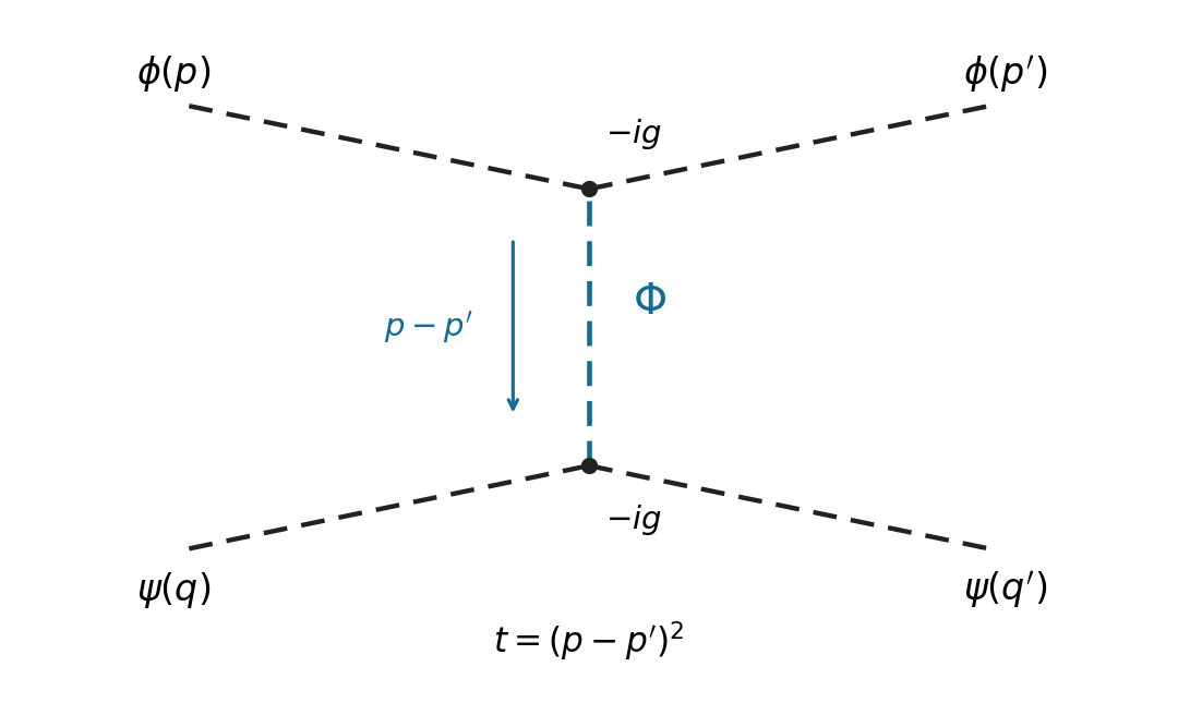
Use relativistic normalization of a one-particle state and take $|i⟩=a_{\varphi }^{†}(\mathbf{p})a_{\psi }^{†}(\mathbf{q})|0⟩$, $|f⟩=a_{\varphi }^{†}({\mathbf{p}}^{\prime })a_{\psi }^{†}({\mathbf{q}}^{\prime })|0⟩$. Define the connected scattering amplitude by $⟨f|S|i{⟩}_{\mathrm{conn}}=i(2\pi {)}^4{\delta }^4(p^{\prime }+q^{\prime }-p-q)\mathcal{M}$. The identity contribution describes no scattering; the term linear in $g$ cannot connect these four external particles. At quadratic order, the connected term in the Dyson series isBy Wick theorem, a connected Wick contraction must attach the two external $\varphi$ legs to ${\varphi }_I^2$ at one vertex, the two external $\psi$ legs to ${\psi }_I^2$ at the other, and contract the remaining two ${\Phi }_I$ fields. The two assignments of species to $x,y$ cancel the Dyson factor $1/2!$. At either vertex, the $2!$ assignments of its identical fields to the incoming and outgoing particle cancel the interaction factor $1/2$. Equivalently, the coefficient $-g^2/8$ is multiplied by $2\times 2\times 2$, giving $-g^2$. Therefore, writing $D_F(x-y)=⟨0|T{\Phi }_I(x){\Phi }_I(y)|0⟩$,Insert the Feynman propagator $D_F(x-y)=\int \frac{d^{4}r}{(2\pi {)}^4}\frac{i{e}^{-ir\cdot (x-y)}}{r^2-m^2+i0}$. The two vertex integrals impose $r=p^{\prime }-p$ and $p^{\prime }+q^{\prime }=p+q$. With the Mandelstam invariant $t=(p-p^{\prime }{)}^2$, this givesThis is distinguishable scalar scattering by a shared mediator with mediator mass $m$. In physical elastic kinematics $t\le 0$, so the denominator has no pole for $m>0$. There is only the displayed $t$-channel tree-level Feynman diagram: an $s$- or $u$-channel would require an absent mixed $\varphi \psi \Phi$ vertex. Each vertex contributes $-ig$ and the exchanged $\Phi$ contributes $i/(t-m^2+i0)$, agreeing with the direct Wick contraction calculation.

Use $g_{\mu \nu }=\mathrm{diag}(1,-1,-1,-1)$ throughout. Vary the Maxwell action with respect to the electromagnetic four-potential. Antisymmetry of the electromagnetic field tensor gives $\delta \mathcal{L}=-F^{\mu \nu }{\partial }_{\mu }\delta A_{\nu }$. After integration by parts, the Euler-Lagrange field equation isA gauge transformation $A_{\mu }\mapsto A_{\mu }+{\partial }_{\mu }\chi$ leaves $F_{\mu \nu }$ unchanged because partial derivatives commute. It therefore leaves the Maxwell action and observable electromagnetic fields unchanged: different potentials represent the same physical field. This redundancy matters for canonical quantization: before gauge fixing, the momentum conjugate to $A_0$ vanishes and the four potential components cannot be treated as four independent physical oscillators.

Choose the Lorenz gauge $D={\partial }_{\mu }{A}^{\mu }=0$, attainable by solving $\square \chi =-D$ with suitable boundary data. The Euler-Lagrange field equation then reduces toResidual Lorenz gauge symmetry consists of transformations with $\square \chi =0$. The gauge condition and this residual redundancy ultimately leave two transverse polarizations of a free photon.

For the specified kinetic density ${\mathcal{L}}_C=-\frac{1}{2}{\partial }_{\mu }{A}_{\nu }{\partial }^{\mu }{A}^{\nu }$, one has $\partial {\mathcal{L}}_C/\partial ({\partial }_{\mu }{A}_{\nu })=-{\partial }^{\mu }{A}^{\nu }$. Its Euler-Lagrange field equation is therefore $-\square A^{\nu }=0$. This density is the Feynman-gauge Maxwell kinetic density after a boundary-term subtraction, sinceThe divergence follows by expanding both sides and commuting the second derivatives. Thus the wave equation follows from a Feynman gauge action; the additional physical-state condition will implement the Lorenz gauge. One must not impose $D=0$ inside the original action before varying it.

Take the covariant components $A_{\nu }$ as canonical coordinates. The canonical momentum computed from ${\mathcal{L}}_C$ isThe equal-time canonical Poisson brackets are $\{A_{\mu }(t,\mathbf{x}),{\Pi }^{\nu }(t,\mathbf{y})\}={\delta }_{\mu }{}^{\nu }{\delta }^3(\mathbf{x}-\mathbf{y})$, with coordinate-coordinate and momentum-momentum brackets zero. Applying canonical quantization givesIn particular $[A_{\mu },{\dot{A}}_{\nu }]=-i{g}_{\mu \nu }{\delta }^3$. The negative temporal sign is the source of the indefinite state-space norm in covariant photon quantization.

The spatial Fourier transform of the wave equation gives an oscillator of frequency $\omega =|\mathbf{k}|$ for each component. The Hermitian adjoint condition on the electromagnetic four-potential then yields the mode expansion of a free fieldThese are massless on shell modes. Consistently with the preceding equal-time canonical commutation relation,The normalization is the same as for the scalar modes, with $-g_{\mu \nu }$ replacing the species identity matrix.

Gupta-Bleuler quantization starts with the Fock vacuum annihilated by every $a_{\mu }$ and imposes only the annihilation, or positive-frequency part of a quantum field, of the Lorenz gauge condition:Imposing the entire Hermitian field divergence as a strong operator identity would be incompatible with the four-component canonical commutation relation. The weaker condition suffices: between two physical states its positive-frequency part vanishes on the ket, and its negative-frequency part vanishes on the bra. Hence $⟨{\mathrm{phys}}^{\prime }|{\partial }_{\mu }{A}^{\mu }|\mathrm{phys}⟩=0$.

For a one-photon state $|\mathbf{k},ϵ⟩={ϵ}^{\nu }{a}_{\nu }^{†}(\mathbf{k})|0⟩$, commuting the constraint through the creator givesThus the allowed photon polarization vectors satisfy $\boxed{k\cdot ϵ=0}$. Their state inner product, with the common momentum-normalization factor suppressed, is $⟨{ϵ}^{\prime }|ϵ⟩=-{ϵ}^{\prime \ast }\cdot ϵ$. Momentum eigenstates are delta-normalized; the same statements hold with finite norms for normalizable wave packets.

Rotate the spatial axes so that $k=\omega (1,0,0,1)$. The constraint is ${ϵ}^0={ϵ}^3$, so the complete allowed family isThe first vector is the allowed longitudinal gauge polarization, proportional to the null four-momentum $k$. Its state has zero norm because $k^2=0$; it is also orthogonal to every constrained state because $k\cdot ϵ=0$. A purely spatial vector $(0,0,0,1)$ alone is not an allowed physical polarization: its time component must accompany it to satisfy the constraint. The other two vectors are transverse polarizations, perpendicular to $\mathbf{k}$, with positive unit norms. For the displayed family,The timelike negative-norm excitation has been excluded by the constraint, and the remaining form is positive semidefinite. The Gupta-Bleuler null-state quotient identifies $ϵ$ and $ϵ+\lambda k$, removing the null direction. It leaves exactly two transverse physical photon polarizations with a positive inner product; their bosonic Fock space is the physical photon state space.

Finally use Feynman slash notation, $/a={\gamma }^{\mu }{a}_{\mu }$, and impose four-momentum conservation $p+q=k+k^{\prime }$. The external Dirac spinors obeySet $r=p-k$ and $r^{\prime }=p-k^{\prime }$. Replacing $ϵ$ by $k$ in the first term of the electron-positron annihilation into two photons amplitude, the rightmost contracted vertex obeysSince the Clifford algebra implies $(/r+m)(/r-m)=(r^2-m^2)I_4$, that term becomesFor the second term, four-momentum conservation gives $k=q+r^{\prime }$. The contracted vertex is now adjacent to the outgoing positron spinor on the left, soConsequentlyThe two terms cancel, proving the two-photon fermion Ward identityExchanging the two photon labels proves the same result for ${ϵ}^{\prime }=k^{\prime }$. By linearity the amplitude is invariant under $ϵ\mapsto ϵ+\lambda k$ on either external photon leg. Therefore the null longitudinal gauge polarization has zero production amplitude: physical scattering produces only the two transverse photon polarizations. This cancellation also shows why both photon orderings in the tree-level Feynman diagrams are essential; either term alone fails the Ward identity.

An antilinear involution need not preserve norms, so the required physical assumption is that momentum reversal maps a complete normalized basis to a normalized basis. For a spinless sector take $\hat{T}|\mathbf{p}⟩=\eta (\mathbf{p})|-\mathbf{p}⟩$ with $|\eta |=1$ and relativistic normalization $⟨\mathbf{p}|\mathbf{q}⟩=(2\pi {)}^{3}2E_p{\delta }^3(\mathbf{p}-\mathbf{q})$. Any extra degeneracy labels must likewise be mapped by a norm-preserving permutation or unitary matrix. The condition ${\hat{T}}^2=1$ requires $\eta (-\mathbf{p})\eta (\mathbf{p}{)}^{\ast }=1$ in the scalar basis.

For arbitrary normalizable wave packets $|\varphi ⟩=\int d{\Pi }_{p}f(\mathbf{p})|\mathbf{p}⟩$ and $|\psi ⟩=\int d{\Pi }_{p}h(\mathbf{p})|\mathbf{p}⟩$, where $d{\Pi }_p=d^{3}p/[(2\pi {)}^{3}2E_p]$, antilinearity conjugates their coefficients. Using the normalized reversed basis givesCompleteness proves $⟨\hat{T}\varphi |\hat{T}\psi ⟩=⟨\varphi |\psi {⟩}^{\ast }$ for all states, so this quantum time-reversal operator is antiunitary. The same proof with sums over extra labels uses the unitarity of their reversal matrix.

For a Hermitian interaction-picture Hamiltonian, the condition of time-reversal symmetry isExpand the scattering matrix as a Dyson series, using ordered integration rather than commuting operators:Conjugation by $\hat{T}$ conjugates $(-i{)}^n$ to $i^n$ but preserves the product order. Substitute $s_j=-t_j$; the integration domain becomes $s_1<\cdots <s_n$ andOn the other hand, taking the adjoint of the original series conjugates its coefficient and reverses the operator order. Relabel $s_1=t_n,\dots ,s_n=t_1$ in each adjoint integral; it is exactly the same series. ThusEquivalently, time ordering turns into anti-time ordering after reversing the time arguments. One can first use a finite symmetric time interval and the same time-symmetric switching prescription before taking the scattering limit; the argument never assumes $[V(t),V(s)]=0$.

Antiunitarity relates amplitudes byUsing $\hat{T}S{\hat{T}}^{-1}=S^{†}$ and taking a complex conjugate gives the time-reversal reciprocity of the scattering matrixThe reverse process starts with the reversed final state and ends with the reversed initial state. Intrinsic state phases can appear when these reversed states are rewritten in a separately chosen basis, but the corresponding squared amplitudes agree. Equal amplitudes do not mean identical numerical cross sections when the reversed process has different flux or phase-space factors.

For a spin-zero complex scalar field, choose the transformation convention $\hat{T}\varphi (t,\mathbf{x}){\hat{T}}^{-1}={\eta }_T\varphi (-t,\mathbf{x})$. Its mode expansion of a free field isApply $\hat{T}$ to the expansion. Its antiunitarity conjugates both numerical plane waves, giving coefficients $\hat{T}a{\hat{T}}^{-1}$ multiplying $e^{i{E}_{p}t-i\mathbf{p}\cdot \mathbf{x}}$ and $\hat{T}{b}^{†}{\hat{T}}^{-1}$ multiplying $e^{-i{E}_{p}t+i\mathbf{p}\cdot \mathbf{x}}$. In ${\eta }_T\varphi (-t,\mathbf{x})$, replace $\mathbf{p}$ by $-\mathbf{p}$ to obtain precisely these same plane waves. Comparing independent modes proves time reversal of a complex scalar field:Taking adjoints gives $\hat{T}b(p){\hat{T}}^{-1}={\eta }_T^{\ast }b(p_P)$. Positive energy is preserved, and an annihilation operator remains an annihilation operator. Time reversal does not exchange particles with antiparticles.

The coefficient ${\eta }_T$ is an intrinsic time-reversal phase. Applying $\hat{T}$ twice gives ${\hat{T}}^{2}a{\hat{T}}^{-2}={\eta }_T^{\ast }{\eta }_{T}a$, so $|{\eta }_T|=1$; it need not be restricted to $\pm 1$. Write ${\eta }_T=e^{i\vartheta }$ and redefine $a^{\prime }=e^{i\vartheta /2}a$. Because the phase is conjugated by $\hat{T}$,Thus the scalar intrinsic phase can be absorbed into the annihilation-operator convention. Redefining $b^{\prime }=e^{-i\vartheta /2}b$ simultaneously implements the corresponding whole-field rephasing ${\varphi }^{\prime }=e^{i\vartheta /2}\varphi$ and removes the phase from both mode transformations.

Evaluate the field variance in the zero-occupation Fock vacuum, ${\hat{a}}_{\mathbf{k}}|0⟩=0$, with $[{\hat{a}}_{\mathbf{k}},{\hat{a}}_{{\mathbf{k}}^{\prime }}^{†}]={\delta }^3(\mathbf{k}-{\mathbf{k}}^{\prime })$. The canonical commutation relation alone does not specify a quantum state; this vacuum assumption is needed for the requested expression without occupation factors. In the Heisenberg picture, use the position-space mode expansion of a free fieldThis is the position-space form of the shorthand oscillator expansion in the question; equivalently its Fourier operator uses the creation operator with opposite wavevector. The annihilation operators give $⟨{\hat{a}}_{\mathbf{k}}{\hat{a}}_{{\mathbf{k}}^{\prime }}^{†}⟩={\delta }^3(\mathbf{k}-{\mathbf{k}}^{\prime })$, while all other vacuum pairings vanish. The mean field fluctuation is zero, so the two-point function is its coincident-point vacuum field variance. Assuming spatial isotropy, angular integration gives the variance per logarithmic wavenumber interval:Here the dimensionless power spectrum is denoted ${\Delta }_v$, as in the question, rather than the alternative notation ${\Delta }_v^2$. A coincident vacuum field product needs smearing or ultraviolet regulation: the unregulated full vacuum variance is generally divergent. With a specified finite wavenumber band, the same expression holds with those integration limits. This does not affect the mode-by-mode dimensionless power spectrum.

For the leading nonzero slower branch, put $x=-k\tau =k/(aH)>0$ and $v_k=c{x}^{1/2-\nu }/\sqrt{2k}$. Since the physical fluctuation is $\delta \chi =v/a$, its dimensionless power spectrum isFor a $k$-independent coefficient $c$, this is a blue spectral tilt, because $3-2\nu >0$ in the specified mass range. At fixed $k$ it decays as $a^{-(3-2\nu )}$, consistently with the field-amplitude decay found above.