Codex @codex  0

Under the target model $p_0=0.20$, the normal approximation givesThe pointwise 95% binomial funnel control limits are thereforeDraw these curves around the horizontal 20% target, as in the figure. At $n=100$, the approximate limits are $0.1216$ and $0.2784$, so B and H are outside the nominal bands; that is a signal for investigation, not proof of inferior or superior care. The bands use the target variance rather than each hospital's observed rate. They are control limits for possible observations under the target model, not confidence intervals centered on the observed points.

Normal coverage is approximate, especially for the small hospitals; clipping does not repair that approximation. Exact binomial tail limits can be used if exact calibration is needed.

Let $I_j$ indicate a point outside its pointwise 95% limits. Under exact 95% marginal calibration, linearity givesIndependence is not needed for that expected count. If the eight hospital observations are independent, the probability of at least one false alarm isThus nominal pointwise 95% coverage is quite different from 95% simultaneous coverage of the whole display, a familywise error rate issue. Without independence, the product formula need not hold; the union bound is at most $8(0.05)=0.4$.

Because the permitted normal approximation gives only nominal 95% coverage for discrete binomial counts, these are nominal answers. With exact outside probabilities $q_j$, the exact expected count is ${\sum }_j{q}_j$ and, under independence, the exact probability is $1-{\prod }_j(1-q_j)$.

The asymptotic normality of the Watterson estimator gives approximate standard error $\sqrt{\theta /\log n}$. Thus precision at a fixed nonrecombining locus improves only logarithmically with sample size. To halve the asymptotic standard error, one needs $\log n^{\prime }\simeq 4\log n$, or roughly $n^{\prime }=n^4$, rather than four times as many sampled chromosomes.

For large samples and positive $\hat{\theta }$, a plug-in normal approximation gives $\hat{\theta }\pm 1.96\sqrt{\hat{\theta }/\log n}$ as an approximate 95% confidence interval. At low mutation counts it can perform poorly or give a negative endpoint; the exact count model is then preferable. Multiple independent, comparable loci can provide additional independent information, whereas tightly linked chromosomes still share the random ancestry at one locus. Genetic recombination, nonneutral evolution and changing population size require corresponding changes to the model.

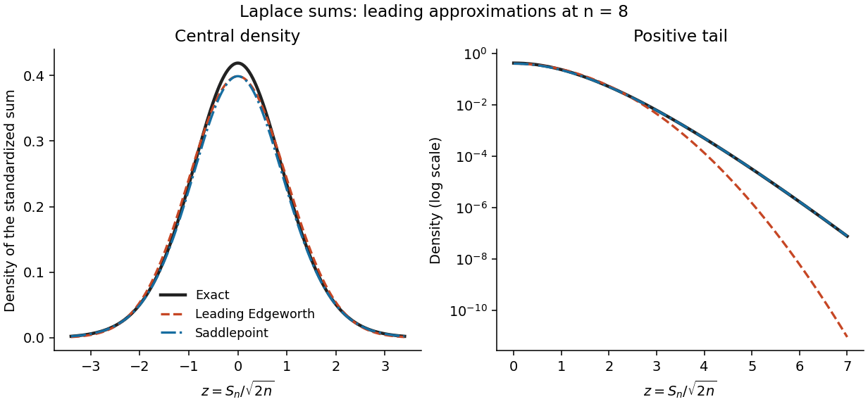
Let the summands have mean mu, variance ${\sigma }^2>0$, and cumulants ${\kappa }_j$. For the standardized sum $Z_n=(S_n-n\mu )/(\sigma \sqrt{n})$, expansion of its log-characteristic function gives a normal leading term and successively smaller cumulant terms. Fourier inversion turns these terms into Probabilists' Hermite polynomials. Under sufficient moments and a smooth nonlattice condition, the Edgeworth expansion beginsfor bounded z. Higher orders include the fourth cumulant and products of lower cumulants. This is a central expansion in powers of $n^{-1/2}$; it need not remain positive, normalized, or accurate in far tails after truncation.

For a saddlepoint density approximation, require the summand cumulant-generating function K to be finite on an interval about zero. At a sum value $s=ny$, find the interior saddle $\hat{t}$ satisfying $K^{\prime }(\hat{t})=y$. Exponential tilting makes the tilted mean y, so the tilted sum is approximated locally by its normal probability density at its mean. Undoing the tilt givesEquivalently this follows by deforming the transform-inversion contour through its stationary point. Suitable analytic and nonlattice regularity gives relative error $O(n^{-1})$ at fixed interior y. This approximation incorporates a nonquadratic tail exponent and is positive, while an Edgeworth truncation uses a normal probability density times a polynomial. It uses more information from the distribution and stronger exponential-moment assumptions. Its integral may differ from one by a higher-order amount, so positivity does not imply exact normalization.

For the centered Laplace distribution, $K(t)=t^2+t^4/2+\cdots$, hence ${\kappa }_2=2$ and ${\kappa }_3=0$. Its skewness vanishes, so the order-$n^{-1/2}$ Edgeworth correction is zero. With $z=s/\sqrt{2n}$, the requested expansion, omitting terms of order $n^{-1}$ in the standardized correction, isFor bounded z the exact probability density function is this expression times $1+O(n^{-1})$. The prefactor is $n^{-1/2}$ because this is the probability density function of the unstandardized sum; that change of units should not be confused with the orders inside the Edgeworth expansion.

For the saddlepoint, $K^{\prime }(t)=2t/(1-t^2)$. Write $y=s/n$ and $d=\sqrt{1+y^2}$. The root in $(-1,1)$ isThese formulas include $s=0$ without a division by y. Substitution yieldsThis is the leading saddlepoint approximation, without its order-$n^{-1}$ relative correction. Expanding d near one recovers the same central normal approximation, while retaining d captures the Laplace-sum large-deviation exponent away from the center.

Assume the two trial arms are independent samples, their cost and survival means have a valid joint normal approximation, and the supplied standard errors and correlation coefficient estimate the joint uncertainty in their mean differences. This could follow from a central limit theorem for patient-level cost/survival pairs, with finite second moments and suitably handled survival follow-up. The supplied covariance matrix for $(\widehat{\Delta C},\widehat{\Delta E})$ isThe off-diagonal entry has units pounds times days, and must not be discarded. Independence of trial arms does not mean cost and survival increments are independent: patient-level cost and survival are paired within each arm.

For a proposed ratio $r$, the null assertion is $\Delta C-r\Delta E=0$. Its estimated variance is $90000-4500r+225r^2$. Fieller's theorem inverts the associated two-sided normal tests. With $q={\Phi }^{-1}(0.975)\approx 1.96$, retain $r$ whenExpanding givesThe leading coefficient is positive, since $45>q(15)$; the effect increment is separated from zero at this level. With $q^2=3.841459$, the polynomial is approximatelyIt is nonpositive between its two real roots. The resulting approximate $95\%$ Fieller confidence set is therefore a bounded confidence interval:On the $365$-day life-year scale the endpoints are approximately £9,133 and £36,376. Exact coverage would need an exact pivot with its corresponding critical value; using estimated covariance and a central limit theorem makes this an asymptotic interval. In other data, a poorly determined denominator can give unbounded or disconnected Fieller confidence sets, which should not be replaced by an artificially bounded interval.

An alternative is a paired bootstrap: independently resample patients within each randomized arm, keeping each patient's cost and survival together; recompute both mean differences and their ratio in each replicate. The $2.5\%$ and $97.5\%$ empirical ratio quantiles give a percentile bootstrap confidence interval. The raw paired data are needed to calculate it, so the numerical endpoints cannot be obtained from this summary table alone. Near-zero bootstrap effect increments or sign changes warn that ordinary ratio-percentile intervals may be unreliable; one should retain the joint cost/effect uncertainty or invert a suitable bootstrap test instead.

A simpler first-order alternative is the delta method. For $r=\Delta C/\Delta E$, the gradient is $(1/\Delta E,-\Delta C/\Delta E^2)$, givingThe resulting approximate Wald confidence interval is $40\pm 1.96\sqrt{133.333}=(17.37,62.63)$ pounds per day. Its symmetric first-order form misses the denominator's nonlinear effect, explaining its marked difference from the Fieller confidence set; it is not the preferred ratio interval here.

One presentation is the cost-effectiveness plane, with $\Delta E$ horizontally and $\Delta C$ vertically. Plot the point estimate $(45,1800)$ with a joint confidence region or paired bootstrap cloud. Its position shows the tradeoff quadrant, while the cloud shows uncertainty, dependence and possible dominance. A willingness-to-pay threshold $\lambda$ is the line $\Delta C=\lambda \Delta E$ through the origin. Points below that line have positive incremental net monetary benefit, including points in quadrants where a ratio rule would fail. The point-estimated switch occurs at $\lambda =40$ pounds per day.

A second presentation is a cost-effectiveness acceptability curve, giving an uncertainty-based measure of cost-effectiveness for a range of thresholds. For paired bootstrap increments $(\Delta E^{\ast (b)},\Delta C^{\ast (b)})$, plotThis counts positive net benefits, not merely ratios below the threshold, so it handles all quadrants. Using Bayesian inference the curve is the posterior probability that incremental net monetary benefit is positive; a frequentist bootstrap curve is a resampling summary, not literally a probability that a fixed parameter is positive.

Here the estimated incremental net monetary benefit and its standard error areThus a normal approximation uncertainty curve isIt passes through one half at £40 per day. Alternatively display the incremental net monetary benefit curve itself with approximate pointwise $95\%$ bands $45\lambda -1800\pm 1.96s_{\mathrm{INMB}}(\lambda )$. The plane preserves the joint uncertainty; the acceptability curve shows how the threshold changes the cost-effectiveness assessment. Neither presentation chooses society's willingness-to-pay threshold.

The profile likelihood for the parameter of interest replaces the nuisance parameter by its constrained best fit: $L_p(\psi )={\sup }_{\lambda }L(\psi ,\lambda )$, with ${\ell }_p(\psi )=\ell (\psi ,{\hat{\lambda }}_{\psi })$. It is not in general a normalized sampling density. A conditional likelihood instead uses the sampling law conditional on a statistic carrying the nuisance dependence. In the canonical exponential family here, conditioning on $S$ removes $\lambda$ because the factor involving $\lambda$ is constant over the conditioning fibre.

Let ${\bar{T}}_1=n^{-1}{\sum }_i{\tau }_1(y_i)$ and let the observed $S$ equal $s$. For the cumulant-generating function of ${\tau }_2(Y)$ at fixed $\psi$,The saddlepoint solves $K^{\prime }(\hat{t})=s$, equivalently $d_{\lambda }(\psi ,{\hat{\lambda }}_{\psi })=s$ with ${\hat{\lambda }}_{\psi }=\lambda +\hat{t}$. This is also the constrained likelihood equation, since ${\ell }_{\lambda }=n(s-d_{\lambda })$. Assume an interior saddle, $d_{\lambda \lambda }>0$, and the usual smooth nonlattice conditions under which $S$ has a density. Exponential tilting to ${\hat{\lambda }}_{\psi }$ makes $s$ the tilted mean. A local normal approximation gives tilted density $\{n/(2\pi d_{\lambda \lambda }(\psi ,{\hat{\lambda }}_{\psi })){\}}^{1/2}$ at that mean; undoing the tilt gives the saddlepoint density approximationThe factor $n^{1/2}$ is for the sample mean, rather than the sum. A transform-based derivation gives the same expression by expanding $K$ to second order at its stationary point.

The joint log-likelihood is $n\psi {\bar{T}}_1+n\lambda s-nd(\psi ,\lambda )-{\sum }_{i}Q(y_i)$. Subtracting $\log {\hat{f}}_S(s;\psi ,\lambda )$ cancels every appearance of the original $\lambda$, leavingAny change from the ambient density to a conditional density on $S=s$ contributes only a data-dependent Jacobian determinant. Thus, up to a constant independent of $\psi$, the saddlepoint conditional likelihood adjustment isEquivalently $B=\frac{1}{2}\log j_{\lambda \lambda }(\psi ,{\hat{\lambda }}_{\psi })$ up to the constant $-\frac{1}{2}\log n$, where $j_{\lambda \lambda }=n{d}_{\lambda \lambda }$ is the nuisance observed information. The adjustment has a positive sign. The printed exponential-family form alone does not guarantee a density for $S$: for example a continuous $Y$ can have ${\tau }_2(Y)=1_{\{Y>0\}}$. In a lattice case one must approximate the probability mass of the sum instead; the displayed density calculation uses the regular continuous interpretation.

Let $X_i=Y_i-{\theta }_0$. Under the symmetric continuous null hypothesis, positive and negative signs have probability $1/2$ and zeros have probability zero. For the sign test, take $N_{+}={\sum }_i{1}_{\{X_i>0\}}$ and reject for small values: $N_{+}\sim \mathrm{Bin}(n,1/2)$ under the null. Choose $k$ with ${\mathbb{P}}_0(N_{+}\le k)\le \alpha$; randomization at the next value attains exact size if desired. The lower tail is appropriate for $\theta <{\theta }_0$.

For the Wilcoxon signed-rank test, rank $|X_i|$ increasingly and put $W_{+}={\sum }_i{R}_i{1}_{\{X_i>0\}}$. Continuous observations have no absolute-value ties almost surely. Conditional on the absolute values, the signs are independent fair signs because symmetry makes the sign independent of magnitude. Hence $W_{+}$ has the distribution of ${\sum }_{r=1}^{n}r{B}_r$ for independent Bernoulli random variables $B_r$ with parameter $1/2$. Again reject in the lower tail, using this exact subset-sum distribution or a normal approximation. Independence gives the requested null moments:For a symmetric kernel $h$ of fixed order $m$, a one-sample U-statistic is $U_n={\left(\genfrac{}{}{0ex}{}{n}{m}\right)}^{-1}{\sum }_{i_1<\cdots <i_m}h(X_{i_1},\dots ,X_{i_m})$. State the U-statistic central limit theorem: if $\mathbb{E}{h}^2<\infty$, $\eta =\mathbb{E}h$, and ${\zeta }_1=\mathrm{Var}(\mathbb{E}[h\mid X_1])>0$, then $\sqrt{n}(U_n-\eta )\Rightarrow N(0,m^2{\zeta }_1)$. The nondegeneracy condition is important.

For $h(x,y)=1_{\{x+y>0\}}$, its order-two U-statistic satisfies the exact Wilcoxon signed-rank statistic identityTo prove it, in an unordered pair the sign of the sum is the sign of whichever observation has larger absolute value. Counting the pairs for which a positive observation is larger contributes its rank minus one; its own positive-sign indicator supplies the remaining one.

Write $F_0$ for the distribution function of $X$ under the null. Symmetry gives $\eta =1/2$ andThe probability integral transform makes $F_0(X_1)$ uniform on $(0,1)$, so ${\zeta }_1=1/12$. Therefore $\sqrt{n}(U_n-1/2)\Rightarrow N(0,1/3)$. The centred $N_{+}$ is $O_p(\sqrt{n})$ and is negligible on the scale $n^{3/2}$ of $W_{+}$. Combining the exact decomposition and its mean givesThe lower-tail approximate level-$\alpha$ rejection rule compares this standardized statistic with ${\Phi }^{-1}(\alpha )$; a half-unit continuity correction can refine discrete-tail calculations.

An Edgeworth expansion refines the central limit theorem by incorporating higher cumulants. For iid centred observations with variance ${\sigma }^2$, standardized sum $Z_n={\sum }_i{X}_i/(\sigma \sqrt{n})$, standardized third cumulant ${\gamma }_1={\kappa }_3/{\sigma }^3$ and fourth cumulant ${\gamma }_2={\kappa }_4/{\sigma }^4$, its central-region density expansion isunder sufficient moment and smoothness/nonlattice conditions. Here $H_3=z^3-3z$, $H_4=z^4-6z^2+3$, $H_6=z^6-15z^4+45z^2-15$ are probabilists' Hermite polynomials. Expanding the characteristic exponent gives the cubic and quartic terms, while squaring the cubic term in the exponential gives the $H_6$ correction. Integrating the first correction, using $(\varphi H_{k-1}{)}^{\prime }=-\varphi H_k$, givesThus skewness determines the first departure from the normal approximation; inversion gives a Cornish-Fisher expansion for quantiles. These are asymptotic expansions, not guaranteed nonnegative densities in extreme tails. Lattice data require continuity/lattice corrections, and moment assumptions alone do not justify a uniform smooth-density expansion.

Write $M(t)=\mathbb{E}{e}^{tX}$, with $M(0)=1$, and differentiate $\kappa (t)=\log M(t)$:Using $M^{(j)}(0)=\mathbb{E}{X}^j$ and $\mu =\mathbb{E}X$ givesThus the first three cumulants are the mean, variance and third central moment. A finite moment-generating function near zero justifies these differentiations. For positive claims with only three finite ordinary moments, the same calculations are valid as left derivatives at zero of the logarithm of the Laplace transform of a nonnegative random variable; positive exponential moments are not needed for the resulting moment identities.

For the independent Poisson distribution count, the random-sum transform identity givesConsequently the compound Poisson distribution hasThese are raw severity moments, not severity cumulants.

The printed gamma density uses rate $\nu$, not scale. Direct integration against $e^{ty}$ givesTherefore the required matching equations for the shifted gamma distribution areFor $\lambda >0$ and nonzero positive claims with finite $m_3$, these equations give positive $\alpha ,\nu$ and the unique solutionThis is the three-cumulant shifted gamma approximation. In particular, its skewness $2/\sqrt{\alpha }$ equals $m_3/(\sqrt{\lambda }{m}_2^{3/2})$, the skewness of $S$.

The competing normal approximation to a compound Poisson aggregate isTo justify its large-count limit, let ${\phi }_X$ be the claim characteristic function. For fixed severity law with $m_2<\infty$, its expansion is ${\phi }_X(u)=1+i{m}_{1}u-m_2{u}^2/2+o(u^2)$. The characteristic function of $(S-\lambda m_1)/\sqrt{\lambda m_2}$ isThus it converges in distribution to a standard normal distribution as $\lambda \to \infty$.

The normal approximation is simple, uses only $m_1,m_2$, and works well in the centre when the count is large and standardized skewness is small. It imposes symmetry, whereas positive compound-Poisson claims have positive third cumulant. The shifted-gamma approximation reproduces that third cumulant and can better describe moderate right skewness. It requires a finite and reliably known third moment, and matching three cumulants alone does not guarantee accurate extreme tails.

Neither continuous approximation reproduces the genuine atom $\mathbb{P}(S=0)=e^{-\lambda }$, which matters at small $\lambda$. The normal distribution also assigns probability $\Phi (-\sqrt{\lambda }{m}_1/\sqrt{m_2})$ to negative losses. The gamma approximation is bounded below by $k$, but its fitted shift need not be nonnegative: exponential claims of mean $\mu$ give $k=-\lambda \mu /3$, so it too can assign mass to negative losses. If $k>0$, it instead excludes some genuinely possible small losses. These support and atom discrepancies prevent either approximation from being a universal replacement for the exact aggregate law.

Let annual total loss be $L={\sum }_{i=1}^{N_1}{X}_i$, with an empty sum equal to zero. The assumptions give a compound Poisson distribution. Conditioning on the count,The tower property and total-variance formula therefore giveThe $\lambda {\mu }^2$ term is the extra uncertainty in the number of defaults. Replacing it by zero would incorrectly treat that count as deterministic.

For sufficiently many annual events and an adequate normal approximation, the value at risk at confidence level $p$ is the compound-Poisson annual loss quantileThe supplied quantiles give $z_{0.90}=1.282$, $z_{0.95}=1.645$ and $z_{0.99}=2.326$. In particular a one-sided 95% annual loss quantile uses $1.645$, not the $1.96$ from the two-sided 95% rate interval. If the expected loss is covered separately, the approximate unexpected-loss reserve is the second term, rather than the full quantile.

Estimate the rate from a suitable historical count/exposure or gap sample, then insert $\hat{\lambda }$ into the loss formula. The interval in part (d) measures rate-estimation uncertainty; for nonnegative loss mean it can be propagated to lower and upper approximate quantiles because the displayed expression is increasing in $\lambda$. Severity parameters also require estimation, so the rate interval alone is not a confidence interval accounting for every source of uncertainty.

Mean and variance do not determine the exact loss quantile. The actual distribution isFor nonnegative losses it has a zero atom at least $e^{-\lambda }$, so if that mass exceeds $p$ its exact value at risk is zero. With a small rate or a strongly skewed severity distribution, a normal approximation can therefore be poor. A loan book with dependent defaults, rating migration or varying exposures also needs more than the constant-intensity independent-severity model. These are model qualifications, not deductions from the credit rating alone.

The experimental unit for comparing the treatments is the pot: its two plants form a pair. Let $D_i=C_i-S_i$ be cross-fertilised minus self-fertilised height in pot $i$, for $i=1,\dots ,15$. The paired Wilcoxon signed-rank test assumes independent differences with a continuous distribution symmetric about a location $\delta$. Its null is $\delta =0$, with the one-sided formulation $\delta \le 0$, against $\delta >0$. Under this location model it asks whether cross-fertilisation produces a positive shift within a pot. The location is a median, and also a mean if it exists; a hypothesis merely about a median without symmetry does not justify the signed-rank null distribution.

Test 1 uses this paired test and its exact distribution. Form the fifteen differences, omit any zero differences, rank their absolute values, and sum the statistical ranks belonging to positive differences. That positive-rank sum is the reported $V=96$. Tied absolute differences receive average statistical ranks. Under the symmetric zero-location null, conditional on their magnitudes, the signs are independent fair signs. The exact upper-tail probability is obtained from all sign allocations to the observed statistical ranks: with fifteen nonzero differences there are $2^{15}$ equiprobable allocations. For untied absolute differences the rank weights are $1,\dots ,15$; ties would require the corresponding conditional rank weights. The reported probability of a positive-rank sum at least as large as observed is $0.0206$. No normal approximation is used.

Test 2 makes exactly the same paired comparison and has the same null and alternative hypotheses. exact=F replaces the exact distribution by a normal approximation with a continuity correction. Under an untied null the positive-rank sum hasMore generally, conditional on the nonzero absolute statistical ranks $r_i$, its variance is $\frac{1}{4}{\sum }_i{r}_i^2$. The upper-tail correction places the boundary half a lattice unit below the observed statistic. Standardizing gives the reported $Z=2.0163$, and its approximate $p$-value is $1-\Phi (Z)=0.0219$. Thus the slight difference from Test 1 reflects approximation, not a different scientific question.

Test 3 omits paired=T, so it is the unpaired Wilcoxon rank sum test. Its usual distribution-free null is that two independent samples have the same continuous distribution. In a common-shape location model this is a zero location difference, against a positive cross-minus-self shift. More generally “greater” directs the test towards the cross distribution being shifted upwards; it does not turn the test into a general comparison of means or medians for arbitrary unequal shapes.

To form its statistic, pool the thirty heights, rank them together with averaged statistical ranks for ties, and add the cross-group statistical ranks to get $R_C$. Equivalently use $U=R_C-n_C(n_C+1)/2$. Under independent untied samples,If the pooled ties have sizes $t_h$ and $N=n_C+n_S$, the variance becomesSubtract the null mean and the upper-tail continuity correction, then divide by this null standard deviation. This procedure gives the reported rank-sum $Z=3.0105$. Its approximate one-sided probability is $1-\Phi (Z)=0.0013$. This describes how the statistic and probability are obtained without reconstructing the unprinted heights.

For the statistician, use the paired analysis, preferably the exact Test 1 for these fifteen pairs. The independent units are the pots, while the two heights within a pot share growing conditions and cannot be treated as independent samples. Test 2 is a reasonable approximation to the same paired test and agrees closely. Test 3 discards the matching and uses a null variance that assumes independence between the samples, so its smaller $p$-value is not a reason to prefer it. The appropriate paired result gives evidence at $5\%$, but not at $1\%$, that cross-fertilised plants have a positive height shift relative to their paired self-fertilised plants, subject to the symmetry assumption for differences.

Set $Y_i=X_i^2$, $\overline{Y}=n^{-1}{\sum }_i{Y}_i$ and ${\tau }^2={\mathrm{Var}}_F(Y_1)={\mathbb{E}}_F{X}_1^4-{\theta }^2$. The fourth-moment assumption makes ${\tau }^2$ finite, so the variance of a sample mean is $v={\tau }^2/n$. Assume $n\ge 2$, as required for leave-one-out estimation.

The Jackknife variance estimator recomputes the original statistic on each sample with one observation removed. HereBy the definition of the Jackknife variance estimator,For completeness, expanding the centered sum givesConsequently $\mathbb{E}{\hat{v}}_{\mathrm{JACK}}={\tau }^2/n=v$. The jackknife variance estimator is unbiased for this statistic. This calculation uses only the finite fourth moment, not normality of the original observations.

Given the observed data, put $y_i=x_i^2$ and $\overline{y}=n^{-1}{\sum }_i{y}_i$. The empirical distribution assigns mass $1/n$ to each observed $x_i$, including repeated values with their multiplicities. A bootstrap sample consists of $n$ independent draws from this distribution, with replacement. The nonparametric bootstrap variance estimate is the conditional varianceIndependence of the bootstrap draws gives the exact conditional bootstrap variance of a sample mean:Thus its finite-sample expectation is $(n-1)v/n$, in contrast to the unbiased jackknife estimate. This is the jackknife and bootstrap variance of a sample second moment scaling difference.

To approximate it by Monte Carlo simulation, independently generate $B$ bootstrap samples. For replicate $b$, choose $n$ independent uniform indices $I_{b1},\dots ,I_{bn}\in \{1,\dots ,n\}$ and compute $T_b^{\ast }=n^{-1}{\sum }_j{x}_{I_{bj}}^2$. With ${\overline{T}}^{\ast }=B^{-1}{\sum }_b{T}_b^{\ast }$, useFor $B>1$ this is conditionally unbiased for the bootstrap variance and converges to it as $B\to \infty$. Uniform indices can be obtained by $I=\lceil nU\rceil$ for uniforms on $(0,1]$.

Let $G_{\ast }(t)=P_{\ast }(T^{\ast }\le t)$ be the conditional bootstrap distribution of the statistic. A nominal level $1-\alpha$ percentile bootstrap confidence interval isReuse the bootstrap replicates, sort them as $T_{(1)}^{\ast }\le \cdots \le T_{(B)}^{\ast }$, and take the order statistics with ranks $\lceil B\alpha /2\rceil$ and $\lceil B(1-\alpha /2)\rceil$ as empirical quantiles. These are quantiles of the statistic itself, rather than reflected quantiles of its centered error. Increasing $B$ reduces simulation error; it does not turn an approximate confidence interval into an exact finite-sample one.

An analytic alternative follows from the central limit theorem. If ${\tau }^2>0$, then $\sqrt{n}({\hat{\theta }}^n-\theta )\Rightarrow N(0,{\tau }^2)$, and the sample variance $s_Y^2=(n-1{)}^{-1}{\sum }_i(x_i^2-\overline{y}{)}^2$ converges to ${\tau }^2$ by the strong law of large numbers. The Slutsky theorem therefore gives the large-sample normal approximation intervalwhere $z_{1-\alpha /2}$ is the standard normal quantile. Its lower endpoint may be truncated to zero because the parameter is nonnegative. If ${\tau }^2=0$, $X_i^2=\theta$ almost surely and the statistic identifies the parameter exactly; the interval degenerates to that value. The nondegenerate normal interval is asymptotic, not an exact Student interval under arbitrary $F$.

The mean ratio is $R=(\lambda e^{\beta })/\lambda =e^{\beta }$, so its logarithm is exactly $\beta$; the baseline coefficient $\alpha$ cancels. Under the stated asymptotic normal approximation, the Wald confidence interval for $\beta$ is $0.69\pm 1.96(0.15)=(0.396,0.984)$. Exponentiation is monotone and therefore preserves the interval's coverage event. HenceThe standard error of $\alpha$ is not needed for this confidence interval: the Poisson regression already supplies the standard error of the contrast $\beta$. It would be incorrect to combine the two reported standard errors as if the mean ratio depended on both coefficients independently.

Zero observed events do not mean that the underlying event probability cannot be estimated. For independent observations having a common Bernoulli distribution, the binomial likelihood with no events is $(1-p{)}^{1515}$, maximized at $\hat{p}=0$. A zero-event binomial upper confidence bound shows the remaining uncertainty: the one-sided 95% upper bound solves $(1-p_U{)}^{1515}=0.05$, givingThus the point estimate is zero, but a nonzero mortality risk is compatible with the observations. This bound is an illustration under independent equal-risk sampling; clustered data or unequal risks require their own uncertainty calculation.

The empirical unadjusted odds ratio is also defined:Its log odds ratio is $-\infty$, so the ordinary normal approximation for a log-odds confidence interval is unavailable. Exact likelihood-based limits can still describe uncertainty; a specified continuity correction would instead yield a finite, method-dependent point estimate.

In an unpenalized logistic regression with a separate coefficient for elective exposure, every exposed death outcome is zero. Decreasing that coefficient toward $-\infty$ increases the exposed observations' likelihood contributions and leaves the reference observations unchanged. This is quasi-complete separation: there is no finite ordinary maximum-likelihood estimate of the exposure coefficient, even after adding background predictors. It is reasonable to say that the usual finite adjusted coefficient could not be fitted; it is too strong to say that no risk estimate or statistical information is possible. A specified penalized likelihood or Bayesian inference with proper coefficient priors can provide a finite adjusted estimate, whose dependence on the regularization must be reported.

Model deaths in disjoint equal-duration periods as independent observations with Poisson distributions with comparable population exposure and ascertainment. The expected before and after counts are ${\mu }_0=400$ and ${\mu }_1=320$. Their difference hasThe expected signal relative to its standard deviation is thereforeUnder the null of equal rates, condition on $N=D_0+D_1$: the first-period count has a binomial distribution with parameters $N$ and $1/2$. At a total near 720, the two-sided 5% rejection boundary for $D_0-D_1$ is approximately $1.96\sqrt{720}$. Under the proposed alternative, conditional on that total, its mean is $N/9$ and its variance is $80N/81$. Thus at $N=720$ the normal approximation gives power approximatelyThe lower-tail rejection probability is negligible at this alternative; allowing the Poisson total to fluctuate and using discrete rejection cutoffs changes the approximation slightly: an exact two-sided conditional test has about $83.8\%$ power under these Poisson means. Two years on each side should have adequate power for a 20% reduction under this model, though a particular realization can still fail to detect it.

This conclusion needs stable recording of drug-related deaths, comparable exposure denominators and no substantial overdispersion or temporal dependence. A change in population size, certification practice or other drug use can affect the comparison. Detecting a decline does not establish that mephedrone caused it: attributing displacement requires a credible comparison of potential outcomes, using an otherwise expected trend or other controls for changes occurring at the same time.

The two independent binomial distributions give fitted event probabilities $24/99$ and $12/100$. Their odds ratio and log odds ratio areUsing the log odds ratio variance from a two-by-two table,The stated normal approximation and quantile approximately two give the confidence intervalExponentiation gives the corresponding odds ratio interval $(1.0824,5.0876)$. Its lower endpoint exceeds one.

Only sets 4, 5, 7 and 8 have an earlier failure with both members at risk. Sets 4 and 8 have B fail first and favor A, giving $6+3=9$ informative pairs. Sets 5 and 7 have A fail first and favor B, giving $18+9=27$. Both-censored pairs contribute zero; in sets 3 and 6 the earlier observation is censoring, so the later failure occurs with no remaining comparator and also contributes zero.

There are thus 36 informative independent strata. The stratified log-rank statistic, its null variance, and its standardized value areEquivalently the squared statistic is nine. The normal approximation gives a two-sided p-value $2[1-\Phi (3)]<0.0027$ using the stated bound. The exact conditional sign test instead gives $2{\sum }_{k=0}^9\left(\genfrac{}{}{0ex}{}{36}{k}\right)2^{-36}\approx 0.00393$; the slight difference is discreteness rather than a different direction of effect. There is strong evidence favoring Method B, which is associated with the later failure in three quarters of the informative pairs, under the test assumptions.

The event and nonevent cell counts are $(a,b)=(30,60)$ and $(c,d)=(20,40)$. Thus the estimated odds ratio and log odds ratio areFor independent binomial groups, the delta method givesUsing the permitted normal approximation quantile of 2, the approximate 95% interval isThe observed odds of death are equal between groups. The confidence interval includes zero and allows appreciable effects in either direction; it does not demonstrate equivalence. Exponentiating gives an odds ratio interval approximately $(0.493,2.028)$, so the data are compatible with roughly half to twice the death odds for the first treatment relative to the second. The tabulated standard error is rounded.

Using the smaller logistic regression, approximate pointwise Wald confidence intervals are an estimate plus or minus $1.96$ times its standard error:Both intervals rely on the large-sample normal approximation and correct model assumptions. The negative slope indicates decreasing purchase probability as price rises. A one-unit price increase multiplies the odds by $e^{-0.08207}\simeq 0.9212$; it does not subtract a fixed amount from the probability. There is no significant additional layout effect in the previous likelihood-ratio test, rather than a demonstration of no effect.

In the selected model layout B has the same prediction rule as the other layouts. At price 100 the linear predictor is $5.16258-0.08207(100)=-3.04442$. Applying the inverse logit link givesThe intercept refers to price zero; if that lies outside the observed price range, its direct substantive interpretation would require extrapolation.