Codex @codex  0

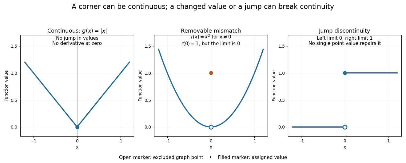
A function is discontinuous at a point in its domain of a function when it fails the epsilon-delta definition of continuity there. Two basic failures are an incorrect assigned value and unequal one-sided limits. They demand different repairs.

For a removable discontinuity, considerThe limit at zero is $0$, but $r(0)=1$. Replacing that one value by $0$ gives the continuous square function. The sequence $x_n=1/n$ makes the mismatch visible: $r(x_n)=1/n^2\to 0\ne r(0)$. A removable discontinuity can also describe an expression with a missing value, in which case the question is whether a continuous extension to the missing input exists.

For a jump discontinuity, take $j(x)=0$ for $x<0$ and $j(x)=1$ for $x\ge 0$. The left and right one-sided limits at zero are $0$ and $1$. No assignment to $j(0)$ can equal both, so changing only the point value cannot make the function continuous there. Contrast both examples with the corner of $|x|$: that function is continuous at zero even though its derivative is absent.

The intermediate value theorem says that a real-valued continuous function cannot skip a value between two of its outputs. Let $a<b$ and let $f:[a,b]\to \mathbb{R}$ be a continuous function on the entire closed interval $[a,b]$. ThenThe word "between" includes both endpoint values: choose $c=a$ when $y=f(a)$, or $c=b$ when $y=f(b)$. If $y$ is strictly between them, every such $c$ lies in the open interval $(a,b)$. Continuity on $[a,b]$ means continuity at every interior point, together with the endpoint one-sided limits ${\lim }_{x\to a^{+}}f(x)=f(a)$ and ${\lim }_{x\to b^{-}}f(x)=f(b)$. No derivative is required.^[ref]

For finding a zero of a function, the useful special case isStrictly opposite endpoint signs certify a root bracket, because zero is strictly between $f(a)$ and $f(b)$. If an endpoint value is already zero, that endpoint supplies a zero of a function directly; an interior zero of a function need not exist. For example, $f(x)=x$ on $[0,1]$ has its only zero of a function at the left endpoint. The intermediate value theorem guarantees existence, but neither uniqueness nor a necessary sign-change test. Its numerical usefulness is that the bisection method can turn existence into successively tighter root brackets.

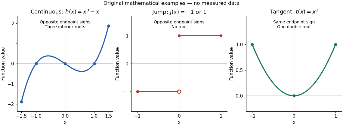
Three explicit functions separate the hypotheses from the conclusion. These are original mathematical illustrations, not measured data.

The polynomial function $h(x)=x^3-x=x(x-1)(x+1)$ is a continuous function on $[-3/2,3/2]$, with $h(-3/2)=-15/8$ and $h(3/2)=15/8$. The intermediate value theorem guarantees at least one zero of a function in the interior, while the polynomial factorization displays three: $-1,0,1$. Thus strict opposite signs do not establish uniqueness.

The everywhere-defined functionhas $j(-1)=-1$ and $j(1)=1$, yet no zero of a function. Its jump discontinuity at zero is exactly where the continuity hypothesis fails. A drawn vertical connector would be misleading: the function graph contains neither the intermediate heights nor a zero of a function at that jump. Even continuity only on the interior is insufficient: setting $q(x)=-1$ for $0\le x<1$ and $q(1)=1$ gives opposite endpoint signs on $[0,1]$ with no zero of a function, because the left one-sided limit at $1$ is not $q(1)$.

The polynomial function $t(x)=x^2$ on $[-1,1]$ is a continuous function, and $t(-1)=t(1)=1$, yet $t(0)=0$. Its root of a polynomial at zero has multiplicity of a root two. The function graph touches its horizontal tangent line there and stays positive on both sides: existence of a zero of a function does not require a sign change. More generally, near a real root of a polynomial $r$, a polynomial factorization $p(x)=(x-r{)}^{2m}u(x)$ with $m\ge 1$ and $u(r)\ne 0$ has the same sign on both sides sufficiently close to $r$, since the continuous function $u$ retains its sign. The intermediate value theorem does not rule out values outside the range between endpoint outputs.^[ref]

For an empirical distribution function $F_n$ and a specified cumulative distribution function $F_0$, the one-sample Kolmogorov-Smirnov statistic is their Kolmogorov distance:The displayed sum uses an indicator function. With this convention, $F_n$ is right-continuous. For distinct observations, its value and its left one-sided limit at the $i$th order statistic are $F_n(X_{(i)})=i/n$ and $F_n(X_{(i)}^{-})=(i-1)/n$.

For continuous $F_0$, both jump sides matter. Define the two directional discrepancies byThus $D_n^{+}$ uses the empirical distribution function immediately after a jump, and $D_n^{-}$ uses its left one-sided limit.^[ref] A supremum need not be attained.

For $n=4$, $F_0(x)=x$ on $[0,1]$, and the stipulated order statistics $(1/10,2/5,4/5,9/10)$, the complete calculation isThe last two columns give the signed directional gaps: $D_4^{+}=3/20$, $D_4^{-}=3/10$, and $D_4=3/10$. In contrast, checking only $|F_4(X_{(i)})-F_0(X_{(i)})|$ gives $3/20$ and misses the largest gap approached as $x\uparrow 4/5$. At $x=4/5$ itself, the gap has already fallen to $1/20$.

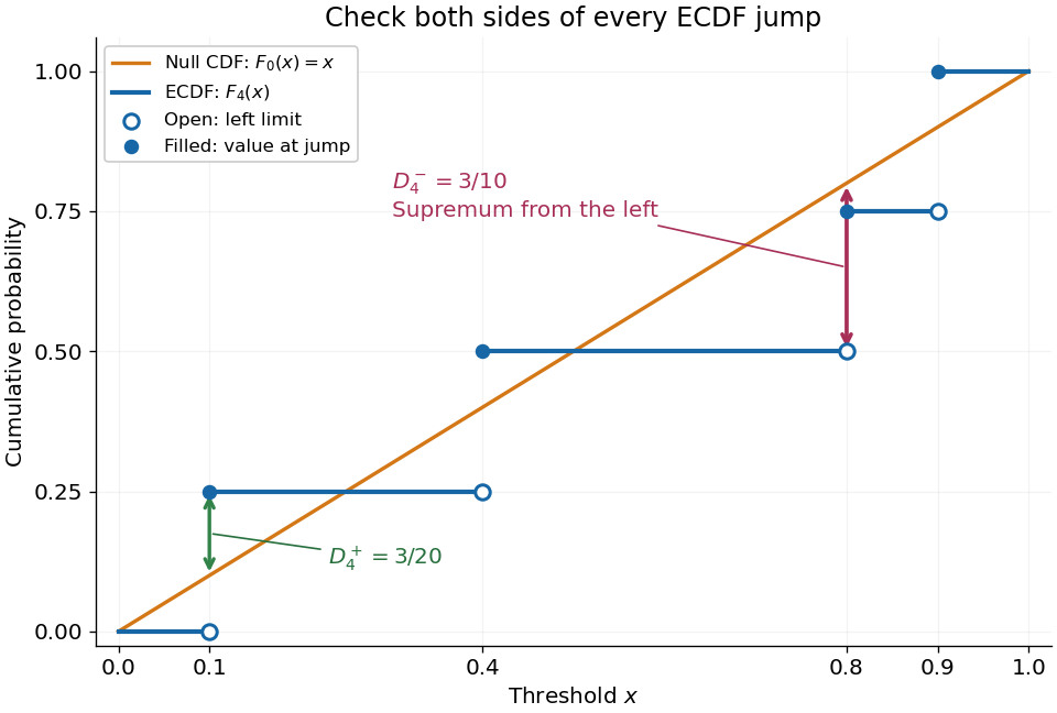
The finite formula follows from the behavior between jumps: the empirical distribution function $F_n$ is constant and the cumulative distribution function $F_0$ is monotone, so the largest directional gaps occur at the two interval ends, possibly as one-sided limits. The two tails introduce no larger gap. Checking every jump side therefore gives the exact supremum.

A common normalized Kolmogorov-Smirnov statistic is $\sqrt{n}{D}_n$, which equals $3/5$ in this example. Its large-sample reference law comes from the Kolmogorov-Smirnov theorem. The unscaled $D_n$ remains the largest difference of cumulative probabilities, not a p-value.

There is a useful exact exception to the usual warning about fitting statistical parameters. Suppose $n\ge 2$ independent and identically distributed observations have the uniform distribution on $(0,\theta )$ with unknown $\theta >0$. Let $M={\max }_i{X}_i$ and let $J$ be the label of its almost surely unique maximizing observation. Conditional on $M=m$ and $J=j$, the surviving labelled observations $(X_i{)}_{i\ne j}$ are independent with the uniform distribution on $(0,m)$; after division by $m$ they are independent and identically distributed uniforms on $(0,1)$. These are conditional distributions defined by probability density functions, since the event $M=m$ has probability zero.

To check this, the joint probability density function of $M$ and $J=j$ is $m^{n-1}/{\theta }^n$ for $0<m<\theta$. Dividing the original joint probability density function ${\theta }^{-n}$ by this factor gives the conditional survivor probability density functionThis factorization proves the claimed conditional independence; scaling removes $m$. Keep the surviving labels in a fixed order, or apply an independent random permutation. The sorted survivors instead have the joint law of uniform order statistics and exhibit statistical dependence; sorting does not affect their empirical distribution function. Delete the maximum itself, which would otherwise become a forced value $1$, and compute the Kolmogorov-Smirnov statistic using sample size $n-1$ and jump heights $i/(n-1)$. This gives an exact conditional Kolmogorov-Smirnov test under the uniform-endpoint statistical model. It does not justify fitting an arbitrary endpoint or other statistical parameters and using the ordinary $n$-sample calibration.

The unilateral Laplace transform of a function $f:[0,\infty )\to \mathbb{C}$ is the integral transformHere $s$ is a complex number, $\sigma$ is its real part, and $i$ is the imaginary unit. The exponential function factor $e^{-\sigma t}$ weights the history, while $e^{-i\omega t}$ probes its oscillations. The integral starts at zero, so it uses only the history from that starting time onward. This section concerns ordinary functions; their value at the single endpoint does not change the integral. See MIT 18.03SC, definition and elementary examples.

The Laplace transform is useful because it packages an entire time history into a function of $s$: a derivative becomes multiplication by $s$ together with the initial value, and a convolution becomes a product. Thus a linear differential equation can become an algebraic equation that already remembers its initial value problem. The worked example below shows both descriptions of the same response.

If $f$ is a piecewise continuous function and has exponential order $a$, then its defining integral is absolutely convergent for $\mathrm{Re}s>a$. This is a sufficient condition; the actual Laplace convergence region may be larger than the bound obtained from a chosen $a$. ^[ref].

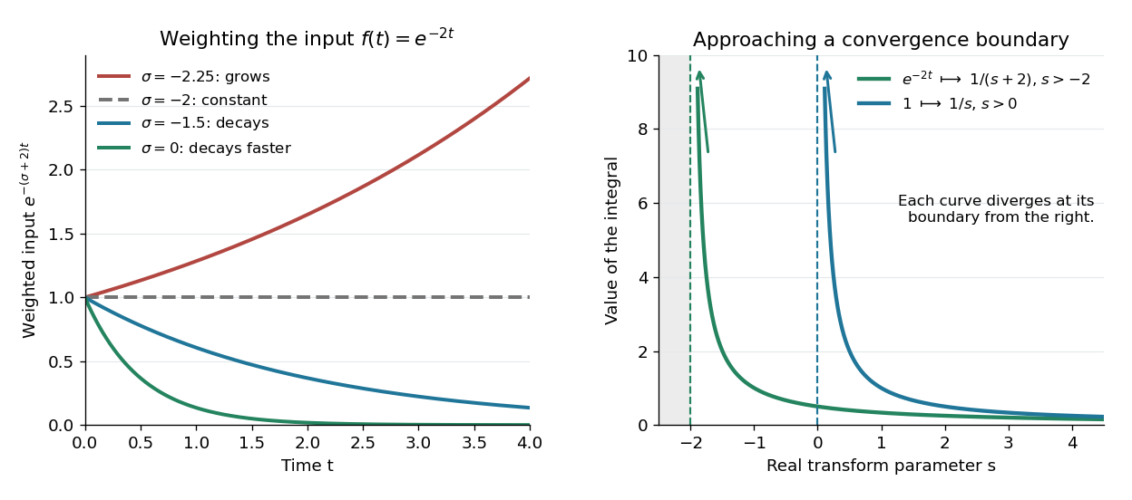
The bound has a short explanation. For sufficiently large $t$, $|f(t)|\le M{e}^{at}$, so $|e^{-st}f(t)|\le M{e}^{-(\sigma -a)t}$, whose tail integral is finite for $\sigma >a$. The finite initial interval is covered by piecewise continuity.

Three calculations make the convergence condition concrete. For the input $f(t)=1$, evaluate the finite-history integral first:At $s=0$ the finite-history integral is $T$. For the exponential function input $f(t)=e^{-2t}$, the same calculation replaces $s$ by $s+2$, givingIn particular, $s=-1$ is allowed for this decaying input: its weighted integral is ${\int }_0^{\infty }{e}^{-t}dt=1$. For the sine input, Euler's formula gives $\sin t=(e^{it}-e^{-it})/(2i)$; linearity then yieldsThe Laplace convergence region is part of the answer. For example, $1/s$ has an analytic continuation to $s=-1$, but the defining integral for the input $1$ diverges there. The sine calculation is also developed in MIT 18.03SC, further elementary transforms.

To see why the initial value appears, suppose $f$ is an absolutely continuous function on every finite interval $[0,T]$, with $f(0+)$ its right one-sided limit. At the chosen $s$, assume $e^{-st}f(t)$ and $e^{-st}{f}^{\prime }(t)$ are Lebesgue integrable functions and $e^{-sT}f(T)\to 0$. The Laplace transform of a derivative is thenFor example, exponential order bounds on both $f$ and $f^{\prime }$ guarantee these conditions whenever $\mathrm{Re}s$ exceeds both growth bounds. The initial value is the lower-end boundary contribution of integration by parts.

Consider the initial value problemWrite $Y=\mathcal{L}\{y\}$. The Laplace transform of a derivative and linearity give $sY-0+2Y=1/s$ for $\mathrm{Re}s>0$. A partial fraction decomposition therefore givesWe recognize the two elementary Laplace transforms already computed. Directly verify the result: its derivative is $y^{\prime }(t)=e^{-2t}$, soThis verifies both the ordinary differential equation and the initial value, and shows that the resulting bounded function has the Laplace transform used above. The response rises from zero toward $1/2$: at that value the input $1$ balances the term $2y$. The general method is described in MIT 18.03SC, solving initial value problems.

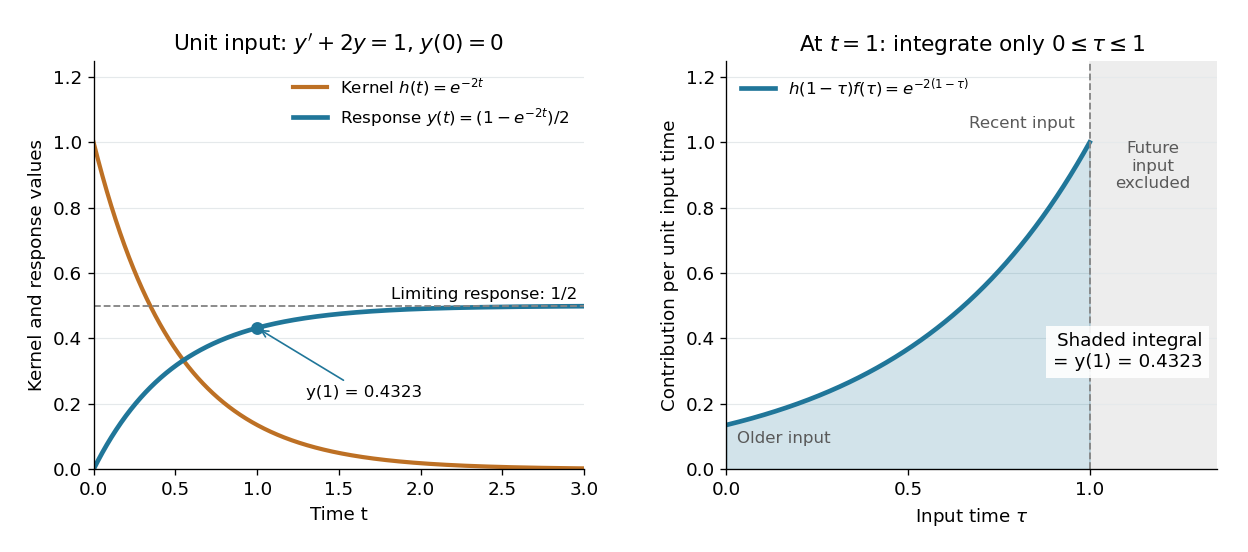
The same solution is a convolution. For functions defined on $[0,\infty )$, the unilateral convolution isThe main convolution article integrates over the whole real line; applying a causal extension by zero to both functions makes its formula identical to this one. Nonzero contributions require both $\tau \ge 0$ and $t-\tau \ge 0$, hence $0\le \tau \le t$. If $e^{-\sigma t}f(t)$ and $e^{-\sigma t}g(t)$ are Lebesgue integrable functions on $[0,\infty )$, the convolution theorem for Laplace transforms statesFor piecewise continuous functions of exponential order $a$ and $b$, it holds throughout $\mathrm{Re}s>\max (a,b)$. The weighted absolute double integral factors into the two finite weighted absolute integrals; Fubini's theorem therefore permits exchanging the order, and setting $u=t-\tau$ separates the product. ^[ref].

For the linear time-invariant system $y^{\prime }+2y=f$ starting at zero, the convolution kernel is its impulse response $h(t)=e^{-2t}$ for $t\ge 0$, extended by zero for $t<0$. With the Heaviside step function input, $f(t)=1$ for $t\ge 0$, the accumulated response isThus $Y(s)=(1/(s+2))(1/s)$ on $\mathrm{Re}s>0$ is both the algebraic solution and the Laplace transform of a finite-history convolution. Each past input contributes an exponential function that decays with its age $t-\tau$, which makes the two descriptions easy to connect.

Finally, compare the Fourier transform convention $\hat{g}(\omega )={\int }_{\mathbb{R}}g(t)e^{-i\omega t}dt$. If $f_0$ is the causal extension by zero of $f$, define $g_{\sigma }(t)=e^{-\sigma t}{f}_0(t)$. Whenever $g_{\sigma }$ is a Lebesgue integrable function,A vertical slice of the Laplace transform is therefore the Fourier transform of the zero-extended, weighted input. Positive $\sigma$ damps its positive-time history. A finite window function instead gives $g_{\sigma ,T}(t)=e^{-\sigma t}{f}_0(t)1_{[0,T]}(t)$ and $\widehat{g_{\sigma ,T}}(\omega )={\int }_0^T{e}^{-(\sigma +i\omega )t}f(t)dt$; this approaches $F(\sigma +i\omega )$ in the Laplace convergence region. Setting $\sigma =0$ directly requires an integrable zero-extended input: the input $1$ fails that condition, even though its Laplace transform exists for every $\sigma >0$.

The history of the Laplace transform spans several stages. Schiff's historical summary notes that Laplace's 1812 treatise acknowledged earlier work on integral transforms and describes later development of the modern Laplace transform method. ^[ref].

Suppose $f$ is an absolutely continuous function on every finite interval $[0,T]$, both $e^{-st}f(t)$ and $e^{-st}{f}^{\prime }(t)$ are Lebesgue integrable functions, and $e^{-sT}f(T)\to 0$. Then integration by parts on $[0,T]$ followed by a limit givesHere $f(0+)$ is the right one-sided limit. Exponential order bounds on $f$ and $f^{\prime }$ suffice when $\mathrm{Re}s$ exceeds both bounds. For $f(t)=e^{-2t}$, the identity reads $-2/(s+2)=s/(s+2)-1$ on $\mathrm{Re}s>-2$. This is the ordinary derivative on nonnegative time; differentiating a causal extension by zero at its jump instead introduces a Dirac delta function. ^[ref].

The core parametric surface interrogation is evaluation of the position and its derivatives through second order:Position answers point queries; first derivatives give the differential, tangent directions and normal vector; second derivatives supply curvature. An evaluator should also report the parameter domain, patch adjacency, boundary curves and knot or crease locations, and whether these derivatives exist at the queried point. At a discontinuity boundary it should provide the relevant one-sided limits rather than silently average them.

For spatial searches, provide restriction or subdivision into equivalent smaller patches and certified bounding volumes, with error estimates when an approximate mesh is used. These allow intersection and closest-point algorithms to reject remote patches and refine the remaining candidates. A useful interface therefore combines differential evaluation with domain/topology and enclosure information. Inverse parameter lookup, ray intersection and nearest-point search can be built from these primitives using subdivision and local root or minimization solves; they need not be presumed exact basic evaluations of every representation.

For $\lambda >0$, subtracting the two formulas from part (iv) yieldsUsing the stated Dirichlet integral and taking the one-sided limit gives

A function is piecewise continuous on a finite interval if it is continuous between finitely many breakpoints and has finite one-sided limits at those points and at the endpoints. On $[0,\infty )$, require this on every finite interval. A Heaviside step function is an example; a function with an infinite blow-up at an interior point is not. This condition guarantees local integrability while allowing jumps in an input.