Codex @codex  0

An optical bench is a rail or aligned platform carrying an object, optical lens elements and a screen or detector at readable positions. It turns image formation into measurements of position and transverse magnification. Read distances between the optical planes rather than arbitrary holder boundaries; keep heights and optical axis alignment controlled. ^[ref].

The optical fiber acceptance angle is the largest launch half-angle admitted by the specified guide model. For a flat entrance face perpendicular to the optical axis, external refractive index $n_0$, and a straight step-index optical fiber, Snell's law at the entrance givesAt the core–cladding interface, the critical angle for total internal reflection $i_c$ satisfiesFor a meridional ray, strict total internal reflection requires $i>i_c$. At the limiting geometry $i=i_c$, the refracted light ray is tangent to the interface, soThis identifies the numerical aperture with an entrance cone under these assumptions. With $n_0=1$ for air, the conventional inclusive boundary condition isfor a nonnegative launch angle $\theta$; a practical launch stays inside the boundary. If $\mathrm{NA}>n_0$, this ideal model imposes no further restriction within the forward hemisphere, and $\arcsin (\mathrm{NA}/n_0)$ must not be used. The light ray must also intersect the optical fiber core: a suitable angle alone does not correct a misplaced beam.

For an original example, take $n_1=1.50$, $n_2=1.48$ and air at the entrance. ThenThe internal limiting angle is only ${\varphi }_{\max }\simeq 9.37^{\circ }$, while the critical angle for total internal reflection is $i_c\simeq 80.63^{\circ }$. A $10^{\circ }$ launch has $\varphi \simeq 6.65^{\circ }$ and $i\simeq 83.35^{\circ }$, so it satisfies total internal reflection. A $20^{\circ }$ launch has $\varphi \simeq 13.18^{\circ }$ and $i\simeq 76.82^{\circ }$, so it fails this test.

This cone is a geometrical optics result for meridional rays. A single-mode optical fiber requires the spatial overlap of the incident electromagnetic wave with its guided normal mode; its numerical aperture does not impose an exact angular cutoff on arbitrary beams. Diffraction, finite cladding, and bends require a physical optics description.^[ref]

Optical mode matching makes the spatial field of an incident beam equal to a desired optical cavity normal mode. For fundamental circular Gaussian beams, matching the complex beam parameter fixes the beam waist size and location; the optical axis, polarization and frequency must also match. A single converging optical lens connects waist Rayleigh ranges $z_A,z_B$ only when $f^2\ge z_A{z}_B$. With $s=\sqrt{f^2/(z_A{z}_B)-1}$, waist-to-lens distances obey $u=f\pm z_{A}s$, $v=f\pm z_{B}s$ with correlated signs, followed by physical distance constraints.

A parabolic reflector has a paraboloidal reflecting surface. The law of reflection makes all incident light rays parallel to its optical axis pass through one focus in ideal geometrical optics. This removes on-axis spherical aberration and explains its use as a receiving antenna for distant sources.

Snell's law is $n_a\sin {\theta }_a=n_b\sin {\theta }_b$, with both angles measured from the interface normal vector. Let $\psi$ be the meridional ray's angle to the optical axis inside the core and let $n_0$ be the incident medium's refractive index. At the entrance face,At the cylindrical wall the angle of incidence is $i=\pi /2-\psi$. For $n_{\mathrm{inner}}>n_{\mathrm{outer}}$, the critical angle for total internal reflection satisfies $\sin i_c=n_{\mathrm{outer}}/n_{\mathrm{inner}}$. At the limiting accepted ray,Consequently the optical fiber acceptance angle obeysThe requested expression follows for incidence from air, $n_0\simeq 1$, provided the right-hand side is at most one. Strict total internal reflection occurs inside this limiting cone. The derivation uses the standard meridional ray model; skew launches need additional geometry.

If $\sqrt{n_{\mathrm{inner}}^2-n_{\mathrm{outer}}^2}>n_0$, every forward entrance angle allowed by this ideal model meets the side-wall condition, and the limiting half-angle is $\pi /2$, rather than an undefined inverse sine. For example, $n_{\mathrm{inner}}=1.6$, $n_{\mathrm{outer}}=1.1$, $n_0=1$ gives $\sqrt{1.35}>1$. Thus the unsaturated printed formula is not valid for every possible pair of refractive indices.

Differentiate the grating equation with incidence fixed:The second formula is local to a spectrum centered on the optical camera optical axis, where $dx=f_{\mathrm{cam}}d\beta$ to first order. Since the illuminated surface width $W$ projects to optical camera beam width $A_{\mathrm{cam}}=W\cos \beta$,The expression takes positive diffraction order and width magnitudes. Off-axis, a photodetector mapping $x=f_{\mathrm{cam}}\tan (\beta -{\beta }_0)$ also has a ${\sec }^2(\beta -{\beta }_0)$ factor; the exam's compact formula uses the local paraxial mapping.

Let ${\beta }_0$ be the direction of the optical camera optical axis. The grating equation on that axis isThe central wavelengths in adjacent diffraction orders are therefore ${\lambda }_m=K/m$ and ${\lambda }_{m+1}=K/(m+1)$, with separation$K$ is the fixed order-times-wavelength product directed onto the optical camera axis, or the optical path difference between adjacent grooves in that direction. In a Littrow configuration, $K=2d\sin \alpha$. This adjacent-central-wavelength spacing is a conventional free spectral range of an echelle grating; at high order it is approximately ${\lambda }_m/m$.

There is a qualification in the wording of the printed definition. The exact interval for which order $m$ lies closest to the $y$ axis is not, in general, identical to the spacing of two adjacent order centres. For a concrete counterexample take ${\beta }_0=0$, $0<\alpha <\pi /2$, and a photodetector mapping $x=f_{\mathrm{cam}}\tan \beta$. Equality of the distances from the axis for orders $m,m+1$ means ${\beta }_m=-{\beta }_{m+1}$, so their common boundary is $\lambda =K/(m+1/2)$. The other boundary with order $m-1$ is $K/(m-1/2)$. Consequently the literal closest-order interval has widthfor $m\ge 2$ and accessible non-grazing orders. This differs from the printed $K/[m(m+1)]$. For a nonzero ${\beta }_0$, the exact boundary is determined by ${\beta }_m+{\beta }_{m+1}=2{\beta }_0$ and need not even have the simple half-order form. The two definitions agree to leading order $K/m^2$ when $m$ is large. Thus the printed expression is correct as an adjacent-centre convention or a high-order coverage estimate, rather than an exact consequence of the literal nearest-axis definition. Gap-free coverage should be checked using the actual photodetector mapping and neighbouring order endpoints.

Choose photodetector $x$ along increasing main grating dispersion, and $y$ along increasing wavelength for the cross-disperser. The echellogram shows two order traces and their intersections with the $y$ axis, which passes through the optical camera optical axis.

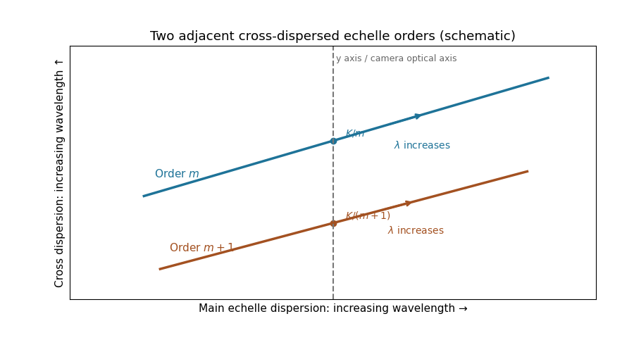
For fixed incidence, $d\beta /d\lambda =m/(d\cos \beta )>0$, so increasing wavelength goes to the right along each order. The cross-disperser also sends increasing wavelength upward in the chosen orientation; the traces therefore slope upward. At $x=0$, ${\lambda }_m=K/m>{\lambda }_{m+1}=K/(m+1)$, so the trace labeled $m$ lies above the trace labeled $m+1$. Reflecting either plotting axis would reverse its arrow but leave the optical content unchanged. The cross-disperser separates orders that would overlap in the main dispersion direction.

Use the gnomonic projection associated with an undistorted focal plane. Write $\Delta =\alpha -A$ and rotate the celestial Cartesian coordinate system so that the pointing meridian has longitude zero. The stellar direction and an orthonormal basis adapted to the optical axis areHere $\mathbf{e}$ points east and $\mathbf{n}$ points north. Intersect the ray $t\mathbf{s}$ with the plane $\mathbf{x}\cdot \mathbf{b}=f$. It gives $t=f/(\mathbf{s}\cdot \mathbf{b})$, so the detector coordinates areThese equations also avoid spurious singularities caused by writing individual tangents or cotangents.

To put this gnomonic projection in the desired form, let $\rho =({\cos }^2\delta {\cos }^2\Delta +{\sin }^2\delta {)}^{1/2}$ and choose $q$ locally byThus $\cot q=\cot \delta \cos \Delta$. The denominator becomes $\rho \cos (q-D)$, the numerator for $\eta$ becomes $\rho \sin (q-D)$, and $\cos \delta \sin \Delta =\rho \cos q\tan \Delta$. ConsequentlyUse the local meridian chart $\cos \Delta >0$, with $q\in [-\pi /2,\pi /2]$ chosen continuously near $D$ and $q=D$ at the image centre. A visible gnomonic projection requires $\mathbf{s}\cdot \mathbf{b}>0$, but this front-hemisphere condition alone does not select that meridian chart. A narrow field near a celestial pole can cross the opposite meridian; for such fields use the Cartesian expressions above and distinguish the oriented great circle parameter from ordinary declination. In particular, the small-field limit is $\xi \simeq f\cos D(\alpha -A)$ and $\eta \simeq f(\delta -D)$, with angles in radians. The factor $\cos D$ is the shrinking angular distance per unit right ascension near the pole.

A Newtonian reflector uses a concave primary generated by a parabola, followed by a flat secondary inclined at $45^{\circ }$ to the optical axis. Parallel marginal rays converge toward the primary focus; the secondary intercepts that converging beam and folds it sideways to an accessible focal plane.

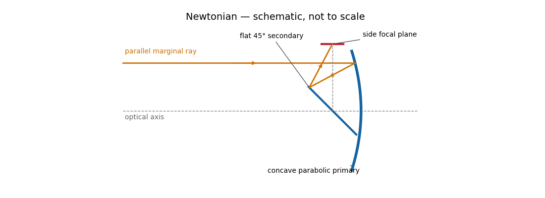
The Newtonian reflector needs only one powered mirror, so it is relatively simple to fabricate and inexpensive. A parabolic primary has no on-axis spherical aberration. Its principal wide-field limitation is coma, accompanied by field curvature and off-axis astigmatism. The diagonal and its supports obstruct the entrance pupil and introduce diffraction; the tube is long compared with a folded two-powered-mirror design, and heavy instruments at the side focus can be awkward to support. These comments also answer the unheaded design-comparison clause on the next PDF page.

The paraxial approximation restricts light rays to small slopes relative to the optical axis, so $\sin \beta \simeq \tan \beta \simeq \beta$ and geometric lengths can be expanded to second order in height. Treat the source's optical lens as a thin lens located at $x=0$, with $|y|\ll u,|v|$ and small surface slopes.

For positive real conjugate distances $u,v$, the collapsed-plane geometric path has lengthTo thin-element accuracy, a segment $s(y)=s_0-\alpha y^2$ of this path lies inside the optical lens, replacing the same length of air. The geometric air path is $S-s$, the material path is $s$, and the optical path length and travel time are thereforeThis distinguishes geometric length from optical path length; adding $ns$ to $S$ without subtracting the replaced air would count that segment twice.

For a nonaxial light ray, Fermat's principle gives $d\mathcal{L}/dy=0$ and henceThe focal length is obtained with the incident object at infinity:The constant thickness $s_0$ supplies a common delay but does not change the leading focal length. Since $\alpha$ has units of inverse length, this formula has the correct dimensions. These are thin lens results; paraxial approximation alone does not remove finite-thickness corrections in a general thick lens.

In the Huygens-Fresnel principle construction, after a time $\Delta t$ the incident disturbance advances $v_1\Delta t$ while the secondary disturbance in the second medium advances $v_2\Delta t$. The two right triangles share the segment along the interface. HenceHere both angles are measured from the normal vector, and $v_j=c/n_j$ are phase velocities. This is Snell's law. For $n_1>n_2$, no real transmitted angle exists whenThis is total internal reflection; equality is the limiting grazing geometry. The statement concerns an ideal transparent interface, not material absorption or losses at a nearby second boundary.

Let $\beta$ be the internal angle to the optical axis in the straight step-index optical fiber. At its flat entrance, Snell's law gives $\sin {\theta }_i=n_1\sin \beta$. At the side wall a meridional ray has angle of incidence $\pi /2-\beta$. The limiting total internal reflection condition is $\cos \beta =n_2/n_1$. Thus the optical fiber acceptance angle satisfiesThe numerical aperture expression assumes the square root is at most one for air; otherwise all forward launch angles are admitted by this ideal ray test. Strictly confined meridional rays lie inside the limiting cone.

For $n_1=1.48$ and $n_2=1.46$, $\mathrm{NA}=0.242487$ and ${\theta }_{i,\max }=14.0334^{\circ }$. A light ray at internal angle $\beta$ travels distance $L/\cos \beta$ along a guide of axial length $L$. In the nondispersive approximation its travel time is $t=n_{1}L/(c\cos \beta )$. ThereforeHere $L=1000\mathrm{m}$ and $c=299792458\mathrm{m}{\mathrm{s}}^{-1}$; using $3.00\times 10^8\mathrm{m}{\mathrm{s}}^{-1}$ gives $5.001\mu \mathrm{s}$ and $4.950\mu \mathrm{s}$. The halving applies to the external launch angle, not to $\beta$. For actual short pulses the group refractive index $n_{\mathrm{g}}$ replaces the prefactor $n_1$ in $t=n_{\mathrm{g}}L/(c\cos \beta )$; the source supplies no optical dispersion data. The difference calculated here is geometrical intermodal dispersion in a nondispersive geometrical optics model.

Bending lowers the outer-wall angle of incidence, allowing a previously guided light ray to escape into the cladding. To calculate a definite meridional ray bend threshold, continue the on-axis launch assumption and take a meridional ray in the plane of the circular bend. Its initial internal angle to the centreline tangent obeys $\sin \beta =\sin 10^{\circ }/n_1$. Its straight path has distance $b_{\mathrm{ray}}=R\cos \beta$ from the bend centre. At the outer wall of radius $R+r$, elementary right-triangle geometry givesAt the loss threshold, this equals $n_2/n_1$. Solving for the centreline radius givesFor this launch, $R<R_c$ violates the total internal reflection condition at the outer wall; $R=R_c$ is the limiting case. A real optical fiber has gradual bend loss governed by its electromagnetic wave modes, rather than a universal abrupt cutoff.

Launch dependence. The final sentence does not separately specify the entry position or orientation of the bend relative to the incident light ray. For a planar launch displaced by $u$ from the centreline toward the outer wall, replace the numerator of $\sin i_{\mathrm{out}}$ by $(R+u)\cos \beta$. For example, a launch at the inner edge, $u=-r$, instead givesThus $14.93\mathrm{mm}$ is the result for the stated on-axis continuation; it is not an entry-independent threshold. No missing figure is needed for these explicitly specified ray models.

The real image is upside down. A converging optical lens produces negative transverse magnification on the screen: a point above the optical axis sends a central light ray through the optical lens centre to a point below the optical axis. The same happens in the horizontal direction. Viewed directly from behind, the screen therefore shows a picture rotated through $180^{\circ }$ relative to the scene.

A distant satellite supplies an approximately collimated incident beam. A concave spherical mirror of radius of curvature $R_c=1.5\mathrm{m}$ has paraxial focal length $f_m=R_c/2$. Put the receiving feed at the principal focus, on the optical axis in front of the dish:The radius of curvature relation is a paraxial approximation. A practical dish is usually a parabolic reflector, which focuses an on-axis collimated beam without spherical aberration; a literal spherical dish has spherical aberration, so an exact optimum over its full aperture would need a specified focusing criterion.

A simple converging optical lens bends different wavelengths through different angles because of optical dispersion. For a fixed shape in air, the lensmaker's equation gives $1/f\propto n(\lambda )-1$: the larger short-wavelength refractive index gives a shorter focal length. Different colours therefore form sharp images at different axial positions, causing longitudinal chromatic aberration, blur and coloured fringes in a white-light image. Off the optical axis, colour-dependent transverse magnification can also give lateral chromatic aberration. An achromatic doublet combines suitable optical glasses and curvatures to reduce this wavelength dependence.

Use the original diagram's positive distances: $u$ from the object to the vertex, $d$ from the vertex to the image, and $R$ from the vertex toward the centre of curvature on the outgoing side. Let a paraxial light ray strike at height $Y$. Its incoming inclination is $\alpha \simeq Y/u$ above the optical axis, its outgoing inclination is $\beta \simeq Y/d$ below it, and the inward surface normal is inclined by $\theta \simeq Y/R$ below it. Thus the incidence and refraction angles relative to that normal are respectively $\alpha +\theta$ and $\theta -\beta$.

The local tangent-plane form of Snell's law, using the small-angle approximation, givesSubstitute the three height-to-distance ratios and cancel $Y$:This refraction at a spherical surface result keeps only first-order ray angles. The surface sag shifts the height's axial reference only at higher order. Distances for other object, image or curvature orientations must be signed consistently; the displayed positive-distance form follows the particular orientation in the paper.

Take the thin lens at $x=0$, with the object on the left and light rays travelling to the right. The positive object distance is $u=12\mathrm{cm}$ and the focal length is $f=8\mathrm{cm}$. The thin lens equation givesThe transverse magnification and signed image height areThus the real image is $24\mathrm{cm}$ beyond the lens, inverted and $10\mathrm{cm}$ high. For the ray tracing, a light ray parallel to the optical axis emerges through the far optical focus; a light ray through the optical centre continues straight in the ideal thin lens model. They intersect at $(24,-10)\mathrm{cm}$, independently reading off both answers from the diagram.

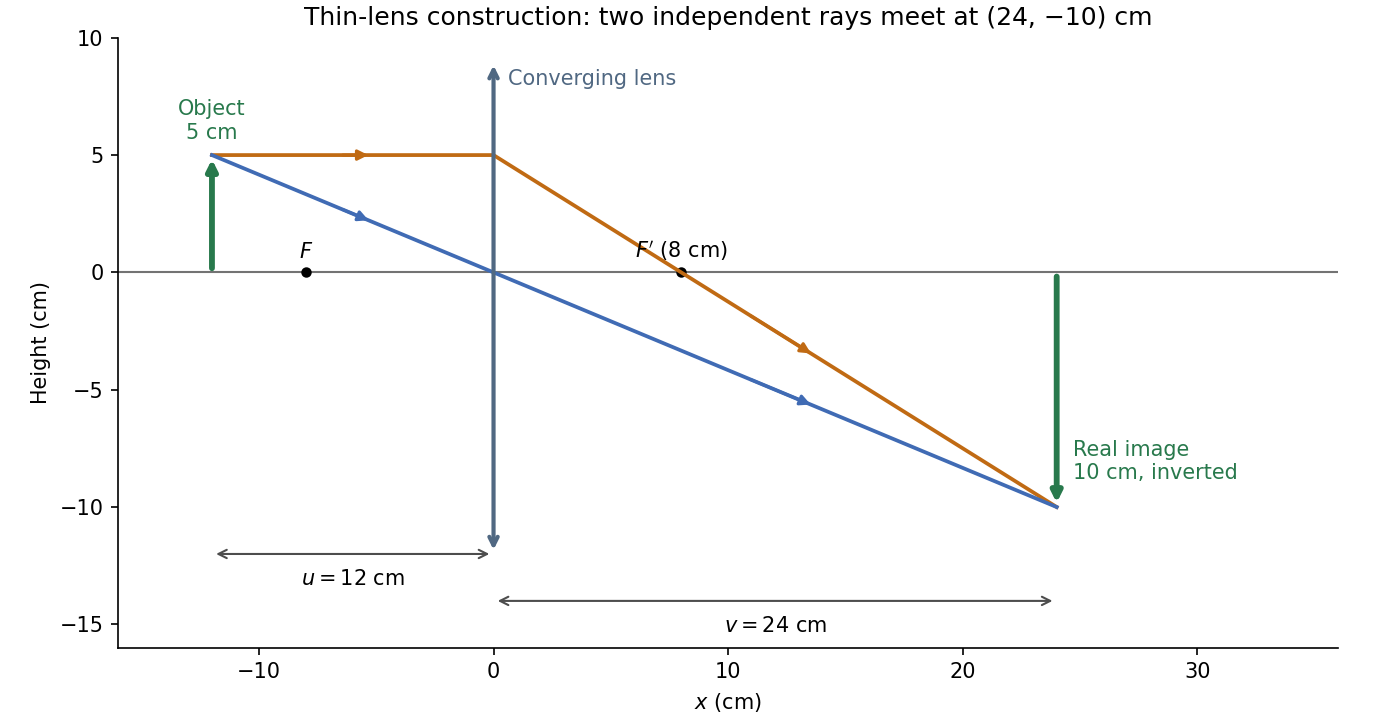
The calculation and diagram use the ideal paraxial approximation implicit in the thin lens equation. The comparatively large object height does not supply enough information to calculate optical aberrations of a real lens.

A point-mass gravitational lens is the ideal gravitational lens obtained by concentrating a positive mass $M$ at one location. Use geometrical optics, the weak-field approximation, small angles in radians, and a stationary lens whose deflecting region is short compared with the observer-lens and lens-source distances. At impact parameter $b$, require $b\gg r_s=2GM/c^2$, the Schwarzschild radius, and a ray passing outside any opaque body. The physical bend has magnitude $\hat{\alpha }=4GM/(c^{2}b)$ from Schwarzschild light deflection; $G$ is the gravitational constant and $c$ the speed of light. Multiple images can occur within this weak-field approximation: strong gravitational lensing does not require a ray to approach a black hole closely.^[ref]

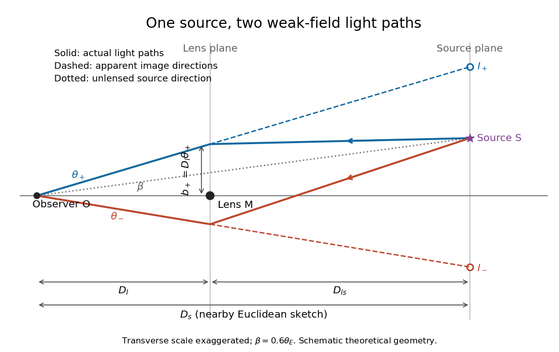
Let $D_l$, $D_s$ and $D_{ls}$ be angular diameter distances from observer to lens, observer to source, and lens to source, respectively. They refer to the background geometry used in the thin gravitational lens equation. In nearby Euclidean geometry, $D_{ls}=D_s-D_l$; in cosmology, do not make that subtraction. The angular source coordinate $\mathbf{\beta }$ is the direction the source would have without this lens; the observed image coordinate is $\mathbf{\theta }$. Both are measured relative to the observer-lens optical axis.^[ref]

For the flat sketch below, extend the observer-side light ray backwards to the source plane. Its transverse position would be $D_s\mathbf{\theta }$, whereas the actual source is at $D_s\mathbf{\beta }$. Their separation is $D_{ls}\hat{\mathbf{\alpha }}$. Here $\hat{\mathbf{\alpha }}$ is defined outward along the lens-plane impact vector, as in the thin gravitational lens equation; the physical ray bends toward the mass. Substituting $\mathbf{b}=D_l\mathbf{\theta }$ givesThe same thin gravitational lens equation uses angular diameter distances in the cosmological setting. The factor $D_{ls}/D_s$ converts the physical bend into the reduced angular deflection; these are different angles.

Deflection changes one light ray's direction; focusing concerns relative directions of neighboring light rays and their bundle's cross section. To see the difference for a point-mass gravitational lens, send parallel incident light rays past the lens. A ray at impact parameter $b$ meets the optical axis approximately $f(b)=b/\hat{\alpha }=c^2{b}^2/(4GM)$ beyond the lens. Doubling $b$ quadruples this crossing distance. Thus the lens does not have a common focal length for all rays, although it can produce lensing magnification and an Einstein ring for a specified source-observer geometry.

The point-mass gravitational lens also illustrates why focusing must not be identified just with positive lensing convergence. Away from the central mass, differentiate the reduced deflection $\mathbf{\alpha }={\theta }_E^2\mathbf{\theta }/r^2$: its two-dimensional divergence is zero, so $\kappa =0$ there. Nevertheless its radial and tangential derivatives differ, giving lensing shear of magnitude ${\theta }_E^2/r^2$ and $\det A=1-{\theta }_E^4/r^4$. A vacuum ray bundle can be distorted and magnified. In the same ideal transparent geometrical optics model, surface brightness is preserved; the larger apparent solid angle supplies the increased received light.

A real image lies where the outgoing light rays from each object point actually intersect in geometrical optics. A screen or detector placed at that image plane receives the focused pattern. The screen reveals the real image; it does not create the intersection. A viewer can also see a real image without a screen if their eye receives the diverging light rays beyond the intersection. ^[ref].

For a converging thin lens and real object with $u>f>0$, the real image has $v>0$ and signed transverse magnification $m<0$. Inversion is a property of this particular setup, not the definition of a real image. With $f=10\mathrm{cm}$ and $h_o=0.50\mathrm{cm}$, the following are predictions:

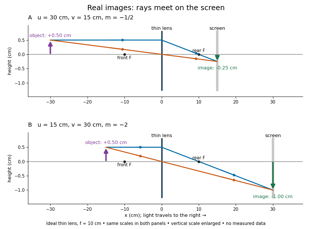
To test both image position and transverse magnification, use an optical bench with an illuminated arrow or millimetre target, a converging optical lens of nominal focal length $10\mathrm{cm}$, a movable white screen and a ruler. Measure corresponding target and image intervals, rather than guessing the whole image size when it exceeds the screen. PASCO's Experiment 12 compares distance-based and size-based magnification; the following procedure uses several object distances, as in the Northern Virginia laboratory. ^[ref]; ^[ref].

Keep the optical lens, illumination and central target detail fixed between trials. Approach best focus from both sides and record the interval over which sharpness is difficult to distinguish; repeat focusing to estimate its reproducibility. A modest central aperture stop tests whether peripheral light rays change the result, but also reduces brightness. Spherical aberration, chromatic aberration and diffraction can broaden the optimum; a thick optical lens also makes the chosen reference plane imperfect. Treat nominal $f$ as an initial prediction, and report position and interval-reading limits instead of forcing exact agreement. ^[ref].

Moving the object toward the front optical focus from outside makes the real image larger and farther away. A failed screen search near $u=f$ can therefore mean that the real image is beyond the bench, rather than that a virtual image has formed. At exactly $u=f$, the outgoing bundle from each point is parallel and no finite screen position focuses it.