Codex @codex  0

Fresnel diffraction retains quadratic aperture-dependent propagation phases and generally depends on both aperture and screen distance. Fraunhofer diffraction neglects those phases and gives the Fourier transform of the aperture in angle space, either sufficiently far away or in a suitable lens's focal plane.

The calculations below use the Fraunhofer, paraxial approximation. For an overall aperture scale $D\sim 1000\lambda$, free propagation requires $L\gg D^2/\lambda \sim 10^6\lambda$. The printed $L\gg 1000\lambda$ alone only makes the separation small relative to distance; it is not by itself the full far-field condition.

In a uniform-field region, $z$ is cyclic and $\gamma$ is constant. Its equation is $d(\gamma m\dot{z})/dt=0$. The radial Euler-Lagrange equation isso with $\dot{\theta }=-\Omega$ and $qB/(\gamma m)=2\Omega$,The radial equation applies on intervals with a regular signed cylindrical-coordinate description; the Cartesian solution handles axis crossings.

In a field-free region, the equations areFor this particle $p_{\theta }=0$, so $\dot{\theta }=0$ and $\ddot{\rho }=0$ outside, until a coordinate change is needed at an axis crossing.

Axial velocity is constant within each uniform region, but not across the ends. In a smooth fringe,The entrance develops an azimuthal speed $|\Omega |{\rho }_0$ while radial velocity remains zero. Conservation of total speed givesForward passage presumes the radicand is positive. The exit fringe changes axial velocity again. Neglecting these small changes is a paraxial approximation, requiring $|\Omega |{\rho }_0\ll v$, rather than an exact consequence of cylindrical symmetry.

Define the positive focusing frequencyIn the paraxial approximation $w\simeq v$, traversal time is $T\simeq l/v$. The exit values areAcross the exit fringe, $p_{\theta }=0$ and $A_{\theta }\to 0$ remove the azimuthal velocity. The radial velocity remains continuous in the thin-fringe model. Outside, the transverse trajectory is therefore straight along a fixed azimuth, not a continuing helix. Taking the outgoing axial speed also as $v$, the distance to the axis isIt is independent of ${\rho }_0$, so all equal-speed paraxial rays focus to a common point. The condition $0<\omega l/v<\pi /2$ ensures the first focus lies beyond the exit. For a weak lens, $\boxed{f\simeq 4({\gamma }_{v}mv{)}^2/(q^2{B}^{2}l)}$.

The relativistic solenoid magnetic lens focuses either charge sign, while its rotation reverses with $qB$. Keeping the exact radius-dependent $w$, or the exit axial-speed change, produces radius-dependent corrections and spoils an exact common focus. Thus the requested focus is appropriately a paraxial result, with the end fields included even when their axial-speed changes are neglected.

The two principal planes are reference planes that represent a centred imaging system in the paraxial approximation. In air on both sides, measure object distance from the front principal plane, image distance from the rear principal plane, and focal length from each principal plane to its corresponding optical focus. They need not coincide with a surface or mechanical centre. Their signed separation matters in the Bessel lens displacement method.^[ref]

The Rayleigh criterion calls two equal, mutually incoherent optical point sources just resolved when one circular-pupil Airy disk's centre coincides with the other's first zero. It is a specified discrimination convention, distinct from full width at half maximum and from precision in estimating one source's position.

For this circular optical pupil, the Rayleigh criterion uses angular separation $s_{\mathrm{R}}={\theta }_1\simeq 1.22\lambda /D$, or $s_{\mathrm{R}}=r_1\simeq 1.22\lambda f/D$ in the paraxial approximation to the focal plane. The point spread functions still overlap.^[ref]

For the Airy disk design example with $D=5.00\mathrm{mm}$, $f=100\mathrm{mm}$ and $\lambda =550\mathrm{nm}$, the angular convention gives $s_{\mathrm{R}}=1.34164\times 10^{-4}\mathrm{rad}$, or about $27.67$ arcseconds, and the image-plane separation is $13.4164\mu \mathrm{m}$. Two equally bright, mutually incoherent optical point sources at separations $0.7$, $1$ and $1.5$ times this scale would have image separations $9.391$, $13.416$ and $20.125\mu \mathrm{m}$ respectively. These calculated cases are compared in incoherent two-source Airy profile.

The Rayleigh criterion is useful because it ties an easily recognized two-peak convention to a predictable optical scale. It does not assert that all information vanishes below that separation. Inferring two unknown positions also depends on photon shot noise, background, unequal brightness and uncertainty in the point spread function; locating a single isolated source is a different task. A theoretical analysis shows that alternative optical measurements can estimate the separation of two incoherent optical point sources below this scale.^[ref]

The mutual optical coherence condition is essential. In incoherent imaging, time-averaged light intensities add. In coherent imaging, wave amplitudes add before squaring, leaving a wave interference term controlled by relative wave phase. Two holes illuminated by the same coherent laser therefore do not implement the equal-incoherent-source convention merely because their individual patterns resemble Airy disks. The coherent single-aperture laboratory test establishes the response of each aperture; it does not establish the pair's mutual incoherence.

With incident light travelling to the right, use positive object distance $u$ to the left, image distance $d$ to the right, and curvature radius $R$ toward a right-hand centre. For a ray hitting at small height $Y$, its incoming inclination, outgoing downward inclination and inward-normal downward inclination are $\alpha \simeq Y/u$, $\beta \simeq Y/d$ and $\theta \simeq Y/R$. The paraxial approximation to Snell's law gives $n_1(\alpha +\theta )=n_2(\theta -\beta )$. Cancelling $Y$ proves the title equation. Virtual conjugates and other centre orientations require corresponding signed distances. Applying the relation at both faces of a thin lens proves the lensmaker's equation.

Consider an original, explicitly normalized model of primary coma, rather than a prescription for a particular optical lens. Let $(u,v)$ be Cartesian coordinates in a circular optical pupil divided by its radius $a$, with $u^2+v^2\le 1$. Let $h=\alpha /{\alpha }_0$ be a signed small field angle divided by an arbitrary positive reference angle. With polar coordinates $u=\rho \cos \theta$, $v=\rho \sin \theta$, prescribe the wavefront errorHere $W_0$ is an arbitrary positive optical path difference scale, not a measured error. The cubic optical pupil dependence and linear field dependence are the classical Seidel form.^[ref]

In the paraxial approximation, light ray direction errors follow the transverse gradient of wavefront error. For a reference sphere a distance $L$ from the exit optical pupil in a uniform image medium of refractive index $n$, the corresponding image-error scale is $s=L{W}_0/(na)$. Choose image-error coordinate signs so the normalized displacement is $\nabla w$; reversing the convention reverses the plotted orientation. Image coordinates below are errors relative to the ideal image of this particular object point, rather than positions of different objects:The partial derivatives explain the asymmetry: opposite optical pupil points $(u,v)$ and $(-u,-v)$ land together, rather than on opposite sides of the ideal image. For $h>0$, every $X$ is nonnegative, while $Y$ can have either sign. The figures stipulate this single wavefront error, omit other optical aberrations and diffraction, and assign no instrument dimensions.

For a ring of fixed optical pupil radius $\rho$, the double-angle formulas for trigonometric functions giveThus each ring maps into a circle of radius $|h|{\rho }^2$ whose centre is displaced by $2h{\rho }^2$. Doubling $\rho$ quadruples both sizes; for $h=1$, the edge ring has centre $(2,0)$ and radius $1$, while the half-radius ring has centre $(1/2,0)$ and radius $1/4$. Superposing these displaced circles produces the comet-like envelope.

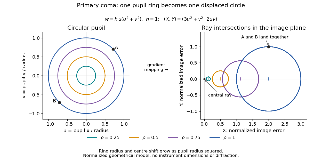
For uniform irradiance over the circular optical pupil, equal area samples give an equal-weight geometrical image. Its centroid is $(h,0)$ because $⟨u^2⟩=⟨v^2⟩=1/4$ and $⟨uv⟩=0$. Moving the coordinate origin to that centroid translates the image; it does not remove its asymmetric shape. Adding a linear term to $w$ likewise translates all light rays equally. These origin choices must be distinguished from changing the optical aberration itself.

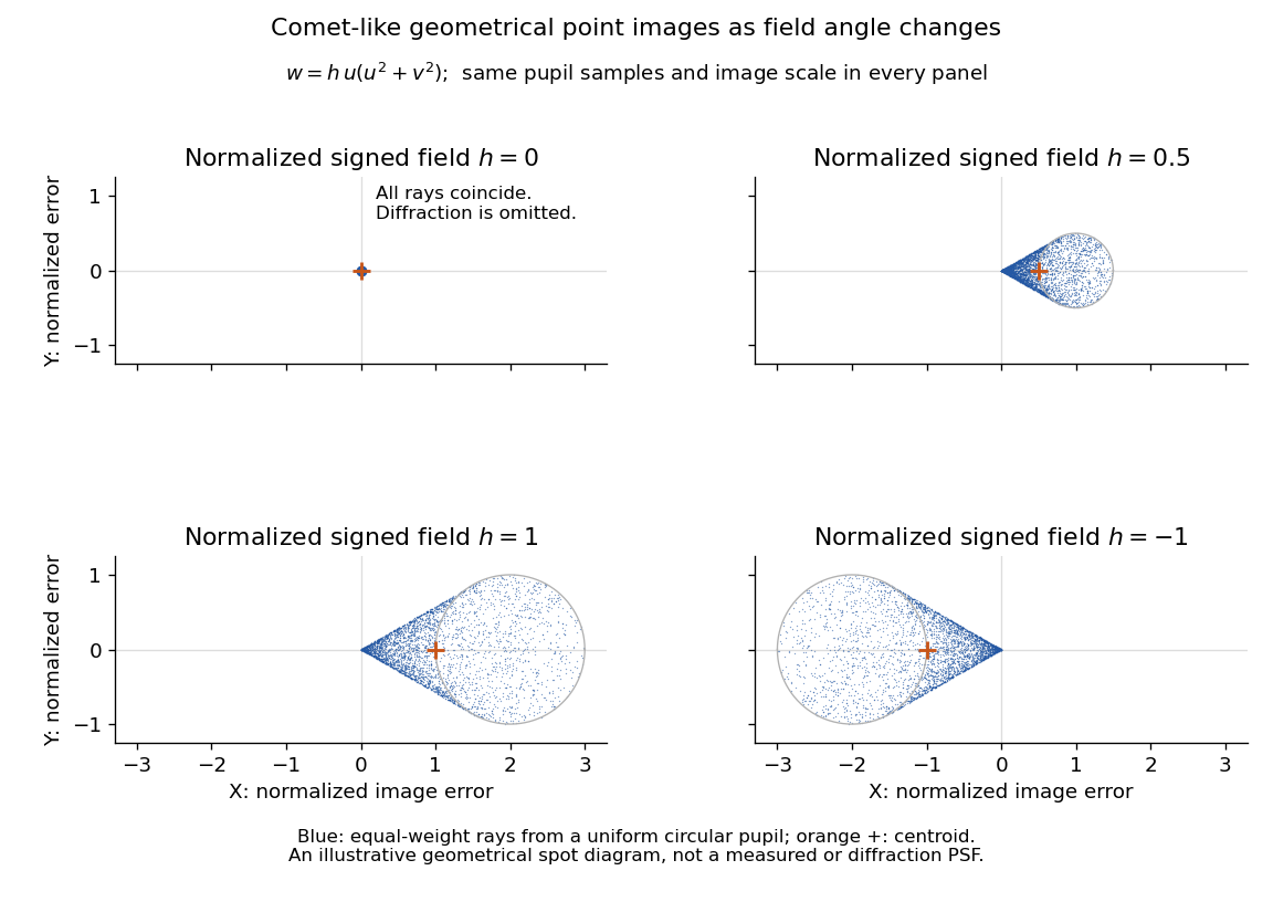
The model's full transverse extent is $3|h|$ along $X$ and $2|h|$ along $Y$. Halving the field angle halves the blur, and reversing it reverses the pattern about the ideal image. This isolates why coma matters for an optical camera's usable field of view: collecting more light does not ensure that off-axis points remain compact. Near diffraction-limited resolution, a physical optics calculation of the point spread function is needed instead of interpreting the geometrical tip as an infinitely sharp image.^[ref]

A spherical lens has refracting surfaces that are portions of spheres, possibly with one plane surface. Their radii of curvature, separation and relative refractive index determine the element's optical power. Rotational symmetry makes the two transverse directions equivalent near the optical axis.

A spherical surface is convenient to manufacture, but does not generally bring every parallel light ray to one point. Comparing focus with the aperture wide open and then reduced reveals spherical aberration: outer and near-axis light rays can focus at different axial positions. The paraxial approximation describes the limiting near-axis behavior.

A thick lens retains the separation of its refracting surfaces when predicting image formation. In the paraxial approximation with air on both sides, object and image distances measured from the respective principal planes satisfy the familiar imaging equation. Measuring instead from one mechanical centre generally introduces an error.^[ref]

A thin lens models an optical lens by collapsing its refracting surfaces into one plane, neglecting thickness relative to the relevant radius of curvature values and object and image distances. Here use an ideal converging thin lens in air and the paraxial approximation: light rays make small angles with the optical axis, so Snell's law can be linearized using the small-angle approximation. Equal surrounding refractive indices on both sides give the familiar symmetric equation.^[ref]

Put the thin lens at $x=0$, with incident light travelling to the right. An object at $x=-u$ has $u>0$. The image coordinate is $x=v$: $v>0$ for a real image and $v<0$ for a virtual image. The converging thin lens has focal length $f>0$, and heights $h_o,h_i$ are signed relative to the optical axis. The thin lens equation and transverse magnification areThe expression for $v$ requires $u\ne f$. Negative transverse magnification means inverted; positive transverse magnification means upright. Remember that the positive distance $u$ differs in sign from the object's coordinate $-u$. ^[ref].

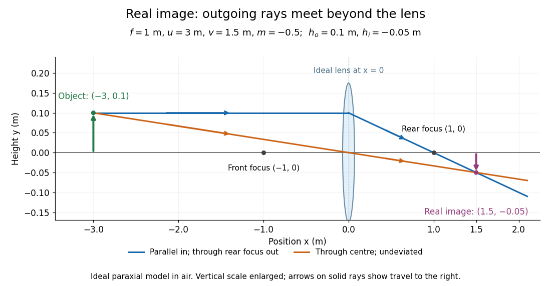
For focal length $f=1\mathrm{m}$, object distance $u=3\mathrm{m}$, and object height $h_o=0.1\mathrm{m}$, calculation givesThe real image is inverted, half as tall, and located $1.5\mathrm{m}$ to the right of the thin lens. A screen at that position receives the image because the outgoing light rays actually meet there.

For the same focal length $f=1\mathrm{m}$ and object height $h_o=0.1\mathrm{m}$, move the object inside the front optical focus, to $u=0.5\mathrm{m}$. ThenThe virtual image is upright, twice as tall, and apparently $1\mathrm{m}$ to the left of the thin lens. Outgoing light rays still travel to the right; only their backward extensions intersect at the virtual image. A screen there cannot collect that image from the outgoing bundle. This geometry explains why a converging optical lens can act as a magnifier when held close to an object. ^[ref].

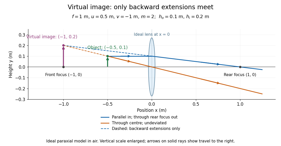
Both diagrams use two rules for ray tracing. A light ray from the object's tip parallel to the optical axis reaches the thin lens at $(0,h_o)$ and exits along the straight line through the rear optical focus $(f,0)$. Another light ray through the centre $(0,0)$ continues undeviated in the ideal thin lens model. Their intersection, or the intersection of their backward extensions, locates the image tip. ^[ref].

A short geometric proof outline makes the signs transparent. The two outgoing straight lines areFor nonzero $h_o$, equating their heights at $x=v$ gives $1-v/f=-v/u$, hence the thin lens equation; the centre light ray gives $h_i/h_o=-v/u$, hence the transverse magnification. This derives the image equations from the ideal ray tracing rules, whose physical justification comes from Snell's law in the paraxial approximation.

At $u=f$, the two outgoing straight lines are parallel: there is no finite image position. For $u>f$ the real image has $m<0$; for $0<u<f$ the virtual image has $m>0$. These cases let an optical camera designer choose a receiving position and let a user understand a magnifier. An actual optical lens has finite apertures, which cause diffraction and impose diffraction-limited resolution; optical aberrations can further blur the image. The diagrams are ideal geometrical optics, with exact coordinates within that model, rather than exact predictions of Maxwell's equations. ^[ref].

The transverse polarization constraint in an angular spectrum requires each source-free electromagnetic plane wave component to have electric field orthogonal to its wavevector in the algebraic sense:For an isotropic homogeneous medium with constant permittivity, this follows by inserting a Fourier component into $\nabla \cdot \mathbf{D}=0$. It restricts the vector fields that can accompany a scalar angular spectrum method calculation.^[ref]

With time dependence $e^{-i\omega t}$ and $\mathbf{k}=(k_x,k_y,k_z)$, the relation becomesWhen $k_z\ne 0$, the longitudinal field is therefore ${\tilde{E}}_z=-(k_x{\tilde{E}}_x+k_y{\tilde{E}}_y)/k_z$. It is not an arbitrary third scalar image that can be propagated independently of the first two.

For an original propagating angular-spectrum component with $\mathbf{k}=k(0.6,0,0.8)$, choosing ${\tilde{E}}_x=1$ and ${\tilde{E}}_y=0$ forces ${\tilde{E}}_z=-0.75$. Polarization along $y$ instead gives a purely transverse-to-axis field for this propagation plane. Thus electromagnetic transversality relative to $\mathbf{k}$ does not require zero field along the laboratory $z$ axis.

For an evanescent angular-spectrum component with $\mathbf{k}=k(1.25,0,0.75i)$, the same choice ${\tilde{E}}_x=1$ gives ${\tilde{E}}_z=(5/3)i$. The dot product is not a Hermitian inner product: there is no complex conjugation of $\mathbf{k}$ in the Fourier-transformed divergence equation. The imaginary longitudinal amplitude represents a phase relationship, not permission to discard the constraint.

At grazing propagation, $k_z=0$, division by $k_z$ fails and the original equation must be used. Boundary conditions, material response and the corresponding magnetic field remain necessary to reconstruct a physical solution. In the strongly paraxial approximation, longitudinal components may be small, but that is an approximation derived from the allowed spectrum rather than a replacement for the vector condition.

Consider two ideal thin electron lenses in successive imaging stages. In each stage choose positive object and image distances $u_i,v_i$ for a real image, measured from its effective lens plane, and neglect the image rotation of a magnetic electron lens. The paraxial approximation givesThe product follows directly by writing $y_1=m_1{y}_0$ and $y_2=m_2{y}_1$. Here $m_i$ is transverse magnification, rather than the enlargement applied later to a photograph. Both inversions cancel in this planar model; actual magnetic electron lenses can additionally rotate the image.

For an original worked example, take $u_1=40\mathrm{mm}$, $v_1=80\mathrm{mm}$, $u_2=50\mathrm{mm}$ and $v_2=150\mathrm{mm}$. ThenA $100\mu \mathrm{m}$ object interval becomes $600\mu \mathrm{m}$ at the screen. The second lens sits $v_1+u_2=130\mathrm{mm}$ after the first. These are calculated distances, not measurements of the 1931 instrument.

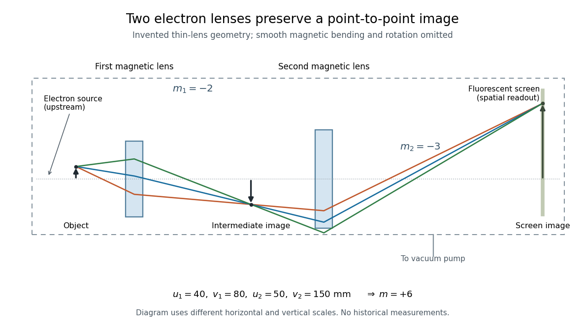
To measure magnification, divide a screen interval between corresponding grid features by the independently known object interval. Repeat over several periods to reduce endpoint uncertainty. For a proposed check, record accelerating voltage, lens electric currents, screen position and specimen orientation; compare one-stage and two-stage images, refocusing as necessary. Changing a lens electric current should change focus and scale, while a blank exposure checks detector background. Keep irradiation and recording enlargement controlled, and repeat the original setting to test drift or specimen damage. These are suggested checks, not a claim that every check was performed in 1931. A grid-scale measurement establishes magnification; resolving much finer features requires a separate target and contrast criterion.

The relevant aperture size $b$ spans the entire coherent array, including the separated elements, rather than one element or a single baseline increment. A quadratic propagation-phase error is small only when $b^2/(\lambda R)\ll 1$ under the paraxial approximation. The often-used boundary $2b^2/\lambda$ is a convention for an allowed phase error, not a sharp physical transition. Individual-element patterns still supply an angular envelope in the far field.