Past exam of the chemistry course of the year 4 of the natural sciences course of the University of Cambridge / 2021 / Interdisciplinary paper IDP1 (Atmospheric Chemistry and Global Change)

Original paper: Released original PDF, physical pages 46–52; printed pages 1–7.

Write $D=[\mathrm{C}{\mathrm{l}}_2{\mathrm{O}}_2]$ and $c=[\mathrm{ClO}]$. In the steady-state approximation for the dimer, chlorine peroxide chlorine peroxide formation is balanced by its two competing removal channels:The association event rate is $k_1[M]c^2$; the associated disappearance rate of chlorine monoxide is twice that value. Each successful photodissociation event produces two chlorine atoms after the subsequent fast fragmentation, and their return to chlorine monoxide consumes two ozone molecules. Thermal dissociation instead returns the dimer to two chlorine monoxide radicals without destroying ozone. Thus the chemical branching fraction for an ozone-destroying event is $f=J_2/(J_2+k_3[M])=0.7$, givingThis is the sunlit chlorine monoxide dimer cycle, with net conversion $2{\mathrm{O}}_3\to 3{\mathrm{O}}_2$. It assumes that the dimer relaxes rapidly, downstream fragmentation and chlorine–ozone reactions are sufficiently fast, and competing chlorine sinks can be neglected. Counting the formation event twice and then multiplying by two again would overestimate loss by a factor of two.

Low temperature favours association into the dimer and, especially, suppresses its thermally activated dissociation back to chlorine monoxide. More of the dimer can therefore follow photodissociation instead of the chemically unproductive thermal return. The supplied branching fraction is a local condition, not a temperature-independent universal yield.

Cold polar air also permits polar stratospheric clouds and efficient heterogeneous conversion of chlorine reservoirs into photolabile forms. The stratospheric polar vortex isolates and cools that air. Darkness permits activation and storage, but rapid catalytic ozone loss requires the return of sunlight. These chemical and meteorological conditions explain the springtime maximum; low temperature alone does not supply the photodissociation photons.

The two initial reservoirs each contain one chlorine atom, so complete activation supplies a total chlorine mixing ratio of $2.2\times 10^{-9}$. Under the specified approximation that active chlorine in sunlight is predominantly chlorine monoxide,The daytime loss is consequentlyFor twelve sunlit hours per day, the daily ozone decrement isThe full-day mean concentration loss is $5.269\times 10^5\mathrm{molecules}\mathrm{c}{\mathrm{m}}^{-3}{\mathrm{s}}^{-1}$. Maintaining that rate would consume the initial ozone in about $79.1$ days. This is a fixed-active-chlorine estimate: reservoir reformation, transport and chlorine partitioning change during a real depletion event, and the approximation fails when insufficient ozone remains to recycle chlorine rapidly.

The initial ozone concentration is $(3\times 10^{-6})[M]=3.60\times 10^{12}\mathrm{molecules}\mathrm{c}{\mathrm{m}}^{-3}$. Over fifty days with twelve active hours per day, the required combined daytime rate isThe mixed chlorine-bromine ozone-loss cycle also consumes two ozone molecules per radical-pair reaction, so $L_{\mathrm{Br}}=2k_6[\mathrm{ClO}][\mathrm{BrO}]$. Subtracting the dimer contribution yieldsThe same result follows by assigning the dimer $1.897$ ppm of the fifty-day loss and the mixed cycle the remaining $1.103$ ppm. This uses the same daylight fraction for both cycles and retains the earlier fixed-ClO approximation. It estimates a sunlit BrO abundance, not the total inventory of bromine in all reservoirs.

Under the proposed steady balance,The air number density cancels from the ratio. ThereforeThe reservoir relaxation test for a chemical steady state gives a hydrogen chloride relaxation time of $1/(k_{10}[\mathrm{OH}])=1.53\times 10^6\mathrm{s}\simeq 17.7$ days. Hydrogen chloride is a reservoir rather than a rapidly equilibrating radical. A steady state is plausible only if chlorine abundance, methane, hydroxyl radical and transport vary slowly compared with several weeks. It is doubtful during rapid vortex breakdown and reservoir reformation, precisely when production and mixing are changing. The numerical hydroxyl radical value is conditional on the steady-state hypothesis, not an independent measurement of hydroxyl radical.

Cooling can increase springtime ozone destruction by extending cold conditions favourable for polar stratospheric clouds, stratospheric chlorine activation and dimer stability. Removal of reactive nitrogen into settling particles can delay chlorine nitrate reformation. With sunlight and substantial available chlorine, the active period can become longer or stronger. Vortex breakup, transport and the declining halogen inventory also matter, so a colder year does not determine the ozone loss by temperature alone.

Outside the cold polar activation regime, cooling generally slows temperature-activated gas-phase ozone destruction and can increase ozone if other conditions are held fixed. This is a weaker, less universal conclusion in the lower stratosphere because transport and imported ozone are important. Enhanced sulfate-surface activation or unusually cold cloud-forming air can instead activate chlorine and reverse the purely gas-phase tendency. Distinguish a local chemical cooling effect from the dynamical response of the midlatitude ozone-column photolysis shielding.

In the upper stratosphere, cooling slows temperature-dependent odd-oxygen destruction, including $\mathrm{O}+{\mathrm{O}}_3\to 2{\mathrm{O}}_2$ and important catalytic reactions. With photochemical production otherwise fixed, the local steady ozone abundance tends to rise. This chemical response is one reason increasing carbon dioxide can enhance upper-stratospheric ozone while cooling that region. It is compatible with enhanced chemical depletion in cold activated polar air; the controlling regimes differ.^[ref]

For fluorine, the key is chemical sequestration, not an inability of free F to react. Fluorine atoms readily form very stable hydrogen fluoride through reaction with hydrogen-containing gases. Breaking hydrogen fluoride or regenerating a sustained free-fluorine radical population under ordinary stratospheric conditions is difficult, so an efficient analogous catalytic family is not maintained.

For iodine, the traditional approximation is limited delivery to the stratosphere. Many iodine source gases are short lived in the troposphere, and their reactive products are efficiently taken up or removed before slow large-scale ascent. This historically motivated omitting iodine from the major stratospheric chlorine/bromine budget. It does not establish that iodine atoms are intrinsically ineffective catalysts, or that stratospheric iodine is exactly zero.

Indeed, the blanket omission needs qualification even for this exam's date. Aircraft observations published in 2020 detected both IO and particulate iodine in stratospheric air and inferred continuing multiphase recycling and ozone loss. Gas/particle partitioning and measurement sensitivity must be considered together; a small gas-phase concentration alone can miss an active reservoir. Thus the traditional supply argument is the intended contrast with fluorine's stable-HF sink, but zero stratospheric iodine chemistry is not supported by those observations.^[ref]

Methane consumes hydroxyl radicals during its initial oxidation and therefore influences atmospheric oxidative capacity and the removal of other trace gases. Subsequent oxidation generates peroxy radicals. In the presence of sufficient nitrogen monoxide, these convert nitrogen monoxide to nitrogen dioxide without consuming ozone, allowing net photochemical ozone production. At low nitrogen monoxide, peroxide formation and ozone-destroying radical reactions compete. Methane oxidation ultimately produces carbon monoxide and carbon dioxide; the sign and rate of the associated ozone response depend on the radical/nitrogen oxides regime, not methane alone.

Methane reaching the stratosphere is oxidized and is an important source of stratospheric water vapor. That water can feed HOx radical family chemistry and alter radiative cooling and polar-cloud conditions. Methane also converts chlorine atoms into hydrogen chloride, opposing some chlorine-driven ozone loss. These effects compete: increasing methane does not have one universal ozone sign at every altitude and latitude.

Methane is an infrared-active greenhouse gas with absorption in the terrestrial thermal spectrum. Its direct forcing is supplemented by chemically induced changes in tropospheric ozone and stratospheric water vapor. Its finite atmospheric lifetime makes sustained emissions and emission pulses different experiments: stopping emissions permits the methane burden to decline much faster than the long tail of a carbon-dioxide perturbation. Quantitative comparisons require a specified emission mass, time horizon and treatment of indirect effects, as formalized by global warming potential.

A humidity assumption is necessary: warming does not by itself specify how much water is available. At fixed relative humidity, the Clausius-Clapeyron equation gives the first-order vapor pressure responseIf water abundance is approximated as proportional to $e_s$, the usual first-order estimate is a $26.7\%$ increase in hydroxyl radical production. Integrating the constant-latent-heat expression instead of linearizing gives $e_s(289)/e_s(285)=\exp [(45050/8.314)(1/285-1/289)]=1.3010$.

There is a small but explicit concentration correction when the square brackets are literal molecules per volume. Since $[{\mathrm{H}}_2\mathrm{O}]=\varphi e_s/(k_{B}T)$ and $P_{\mathrm{OH}}=2k[\mathrm{O}({}^{1}D)][{\mathrm{H}}_2\mathrm{O}]$,The corresponding finite-change concentration result is $(285/289)(1.3010)-1=0.2830$. The $25.3\%$ linear concentration estimate and the $26.7\%$ vapor pressure approximation express different stated approximations; neither follows without a humidity condition.

Extra water increases the fraction of oxygen singlet D atoms reacting to form hydroxyl radicals rather than being collisionally quenched and recycled into ozone. In clean, low-nitrogen oxides air this tends to increase ozone loss. In nitrogen oxides-rich air, increased hydroxyl radical can accelerate precursor oxidation and ozone production, while radical termination also changes. Greater hydroxyl radical production therefore does not imply a universally positive or negative ozone response.

The lost ozone-column photolysis shielding is $\Delta N=20(2.69\times 10^{16})=5.38\times 10^{17}\mathrm{molecules}\mathrm{c}{\mathrm{m}}^{-2}$, so its optical-depth decrement is $\sigma \Delta N=0.0538$. Under the stipulated effective-cross-section Beer-Lambert model, the transmitted photodissociation flux increases by $\exp (0.0538)$.

The short-lived oxygen singlet D atom satisfies $[\mathrm{O}({}^{1}D)]\simeq J_{{\mathrm{O}}_3}[{\mathrm{O}}_3]/(k_q[M])$ when quenching dominates. At fixed local ozone, water and air density, hydroxyl radical production is proportional to $J_{{\mathrm{O}}_3}$. ConsequentlyA linear optical-depth approximation would give $5.38\%$. A realistic calculation integrates the wavelength-dependent absorption cross section, quantum yield and actinic flux; clouds and multiple scattering modify the simple transmitted-beam model.

Ozone change can also alter the radiative temperature structure, water vapor and circulation, thereby changing the water reaction channel and the supply of ozone/precursors to the troposphere. If the held-fixed tropospheric ozone assumption is relaxed, altered ozone itself changes the photochemical source of oxygen singlet D atom. These are additional feedbacks, distinct from the isolated UV-transmission calculation above.

For the tropospheric OH budget, let $P$ be hydroxyl radical production per unit volume and $K$ its total first-order loss frequency. The present hydroxyl radical steady state hasHere one year is $365.25$ days; using it consistently makes the reported lifetimes in years independent of that conversion convention. Methane's chemical lifetime is ${\tau }_0=1/(k_2[\mathrm{OH}{]}_0)$, givingThe current combined loss frequency already includes existing hydrogen, so add only the incremental hydrogen sink:Holding production and the other losses fixed then gives $[\mathrm{OH}{]}_1=5.107\times 10^5\mathrm{molecules}\mathrm{c}{\mathrm{m}}^{-3}$ andThe rapid hydroxyl radical adjustment time, $1/K$ of order a second, supports its steady-state approximation in this box model. Subsequent methane growth would itself change hydroxyl radical consumption, so the computed increase is not a fully coupled long-term atmospheric prediction. Detailed molecular hydrogen modelling treats changes in methane, ozone and stratospheric water alongside reductions in other precursor emissions.^[ref]

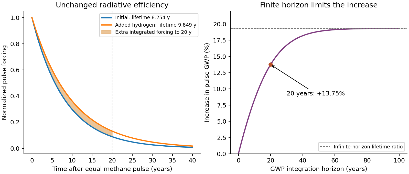
The finite-horizon GWP lifetime sensitivity follows because a longer lifetime leaves more methane from a given pulse at later times and raises the steady burden for a given constant emission rate. For the stipulated exponential pulse response and unchanged greenhouse gas radiative efficiency, the integrated methane forcing over horizon $H$ is proportional to $\tau (1-e^{-H/\tau })$. The same carbon dioxide reference pulse appears in both global warming potential denominators, so it cancels from their ratio:Thus the twenty-year GWP increases by $13.75\%$ under these fixed-efficiency assumptions. This is smaller than the $19.33\%$ lifetime increase because part of the extra forcing occurs beyond the finite horizon. For an infinite horizon the fractional increase would approach the lifetime ratio. Indirect forcing and the distinction between a chemical lifetime and a hydroxyl radical-coupled methane perturbation lifetime require a fuller chemical model; they are held fixed in this comparison.

Lower carbon monoxide and VOC emissions generally reduce the supply of peroxy radicals from their oxidation and therefore reduce photochemical ozone production where nitrogen monoxide is available. Lower nitrogen oxides abundance suppresses the nitrogen monoxide-to-nitrogen dioxide pathway in NOx-limited ozone production regions. These are reasons for a regional/background ozone decrease when fossil-fuel precursor emissions decline.

The response can have the opposite local sign in a nitrogen monoxide-rich urban core: reducing nitrogen monoxide weakens ozone titration, and reducing nitrogen oxides in a VOC-limited ozone production regime can initially lessen radical termination and raise ozone. Less carbon monoxide can also leave more hydroxyl radical available to remove methane, partly opposing the hydroxyl radical demand from leaked hydrogen. Changes in precursor transport, chemistry and sunlight matter. Reduced emissions usually reduce net regional ozone production, but do not guarantee a lower ozone concentration at every monitoring site.

Absorption depends on an allowed transition with a nonzero transition dipole moment and appreciable line strength at wavelengths carrying terrestrial thermal radiation. Molecular vibration and molecular rotation, level populations and pressure/temperature-dependent line shapes determine the spectrum. A band in an atmospheric window can be more effective incrementally than one already strongly absorbed by water or carbon dioxide. Symmetry can make a vibration infrared inactive even when the molecule has many normal modes. Atmospheric lifetime affects the persistence of a released gas, not the intrinsic absorption strength of one molecule.

The size parameter $x=2\pi r/\lambda$, complex refractive index and particle shape determine scattering strength and direction. In the small-sphere Rayleigh scattering regime, scattering cross-section scales as $r^6{\lambda }^{-4}|(m^2-1)/(m^2+2){|}^2$; the Mie scattering regime is needed when particle size approaches the wavelength. Particle number density and particle size distribution, aerosol hygroscopicity and the angular fraction returned to space control an ensemble's radiative effect. High scattering does not imply strong cooling if most light is scattered forward or the particle also absorbs strongly; single-scattering albedo distinguishes scattering from absorption.

Carbon dioxide is relatively well mixed, its abundance is measured accurately, and its spectroscopy and large-scale radiative effect are well constrained. Aerosols are short lived and spatially heterogeneous; uncertain emissions, removal, size, composition, water uptake and height change both scattering and absorption. Their aerosol-cloud interaction effects and subsequent cloud adjustments add uncertainty, and the unobserved preindustrial aerosol baseline complicates anthropogenic attribution. Thus total aerosol forcing combines poorly constrained physical pathways and a less certain counterfactual, rather than simply an uncertain molecular absorption coefficient.^[ref]

Injected sulfur dioxide is oxidized, principally through hydroxyl radical chemistry, to sulfuric acid, which nucleates or condenses into aqueous sulfate particles. A suitably sized, weakly absorbing particle population scatters some incoming sunlight back to space, increasing planetary albedo and decreasing absorbed solar energy. The sulfur dioxide molecules are precursors, not the persistent reflective population.

The albedo lifetime reflects aerosol formation, growth/aerosol coagulation, sedimentation, stratospheric transport and eventual return to efficiently scavenged tropospheric air. The stratosphere has little atmospheric precipitation, so the effect can outlast analogous tropospheric aerosol. The assumed year is an effective persistence scale, not a universal lifetime of sulfur dioxide oxidation or an exact clock for every particle.

For the albedo-to-forcing conversion, Earth intercepts sunlight over a disk but distributes the global mean over its full sphere, giving incident mean flux $S_0/4$. The absorbed shortwave flux is $F_{\mathrm{abs}}=(1-A)S_0/4$, and henceThe cooling magnitude is $1.37\times 10^{-5}\mathrm{W}{\mathrm{m}}^{-2}$ for the assumed one-year effect of one mass unit of injection. Albedo does not change the sunlight incident at the top of the atmosphere; it changes the absorbed/net incoming flux. The minus sign therefore accompanies the radiative cooling.

For the first year's increase, the forcing increment isUsing linear superposition of the supplied one-year aerosol calibration,This compensates the year-end forcing increment for a one-year aerosol effect. It is not a one-time permanent cancellation of the continuing carbon-dioxide increase. Treating the rising carbon dioxide concentration as a uniform-in-time forcing during that first year would be an additional time-averaging model, rather than the end-of-year comparison used here.

If “steady temperature in 2050” means preventing the next annual increase relative to the climate at the delayed start, the relevant forcing increment isIts smaller value follows from $dF/dC=5.4/C$: the same additional ppm gives less incremental forcing at a higher baseline.

That interpretation must be separated from the earlier objective of holding temperature at the original reference climate. To cancel the accumulated increase from $415$ to $500$ ppm requiresThis annual versus accumulated radiative forcing distinction is essential: the first box offsets just the further year's growth; the second is the equivalent one-year aerosol inventory needed for the accumulated forcing. In subsequent years that inventory must be replaced as particles disappear and increased as carbon dioxide rises. A delayed start does not erase the earlier warming merely because the annual incremental requirement is smaller.

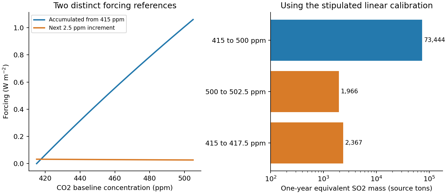
The logarithmic forcing relation implies decreasing incremental forcing per additional ppm, explaining the two annual-increment results. It does not imply that a higher total carbon dioxide burden requires less compensation relative to a fixed original climate. The chosen reference and whether an end-of-year, mean-year or steady maintained aerosol burden is intended must remain explicit.

The numerical mass estimates use an unusually simple, stipulated constant albedo-per-mass calibration. Real particle size and lifetime change with loading, aerosol coagulation, injection altitude/latitude and circulation. Sulfate absorbs radiation as well as scattering it and changes stratospheric chemistry. A global-mean shortwave/longwave radiative forcing balance also need not reproduce regional temperature, rainfall or transient ocean heat uptake; it does not undo CO2-driven acidification. Chemistry–climate simulations explicitly resolve some of these competing aerosol-size, temperature and ozone effects.^[ref]

Use the transmitted-flux form of the Beer-Lambert law. The optical depth falls from $0.25$ to $0.225$, soA ten-percent loss of ozone therefore does not imply a ten-percent increase of transmitted UV. The response depends on the initial optical depth, wavelength and path geometry. This calculation uses the stated effective optical depth and holds the incident flux and other absorbers/scatterers fixed.

For independent first-order sinks acting on the same well-mixed burden, loss frequencies add:The fraction converted to sulfate before removal by the competing direct-deposition sink isThe individual event fractions are $0.40$ for direct sulfur dioxide deposition, $0.40$ for cloud oxidation and $0.20$ for hydroxyl radical oxidation. These are branching fractions for the sulfur dioxide fate; sulfate formed by oxidation can subsequently be deposited as well. The argument assumes the supplied channel lifetimes are compatible effective first-order rates, not residence times of isolated air masses that never exchange.

First, weakly absorbing sulfate scatters shortwave electromagnetic radiation and tends to cool the surface/planetary energy budget, with magnitude and sign influenced by cloud background and particle optics. Second, sulfate can supply cloud condensation nuclei: at fixed cloud water, more activated droplets give smaller droplets and greater cloud albedo through the Twomey effect; atmospheric precipitation and water-content adjustments can modify that idealized cooling. Third, sulfate particles change atmospheric composition through uptake, aqueous chemistry and heterogeneous surface reactions, with their acidity and available reactants controlling what is converted. Particle surfaces alone do not guarantee polar-style stratospheric chlorine activation in an ordinary tropospheric cloud.^[ref]

Increasing greenhouse gases generally strengthen the wave-driven Brewer-Dobson circulation: tropical stratospheric upwelling, poleward transport and extratropical descent intensify in model projections. This can shorten transit times, reduce tropical lower-stratospheric ozone by importing ozone-poor air, and increase ozone supply to extratropical regions or the troposphere. Changes in wave propagation and momentum deposition drive the residual circulation; it is not simply a direct thermal overturning inferred from local temperature alone. Regional branches and variability need not all accelerate equally.^[ref]

At fixed precursor emissions, more tropospheric water vapor in a warmer climate promotes the ozone-photolysis/O(${}^{1}D$)-water loss route, especially in clean tropical lower air. Warmer conditions also accelerate some precursor chemistry; lightning nitrogen oxides, stagnation and stronger stratosphere-to-troposphere ozone transport can increase ozone elsewhere. Thus near-surface regional ozone and the integrated tropospheric burden can respond differently. There is no universal decrease of the global burden from the humidity effect alone; competing chemistry and transport must be evaluated consistently.

For the chemical sink, ${\tau }_{\mathrm{C}{\mathrm{H}}_4}\sim 1/(k[\mathrm{OH}])$. Warming increases the methane–hydroxyl radical rate constant and, with increased water vapor, often increases hydroxyl radical production, tending to shorten the chemical lifetime. Changes in ozone photodissociation, radical recycling, lightning and competing carbon monoxide/VOC/methane consumption can reinforce or oppose that trend. Increasing methane itself consumes hydroxyl radicals and lengthens its methane perturbation lifetime. The physical/chemical warming tendency should therefore be separated from scenarios with changed emissions; shorter chemical lifetime at fixed precursor conditions is a tendency, not an unconditional prediction for the future atmosphere.^[ref]