Solutions to all three questions of the University of Oxford Part A examination of 16 June 2015, printed as “Waves and Fluids.” Source: released examination archive, member
FOI-20210708-1 - Data/a13760w1.pdf, printed pages 1–3. Question statements are omitted. Oxford's published solutions policy excludes this odd-numbered year, and a bounded exact-paper search found no advertised full or partial answers.Write the planar velocity field as , with . Expanding the curl givesConsequently, for a piecewise smooth path from the origin to ,The arbitrary additive constant may be set to zero. The integrand is exactly , so the fundamental theorem for line integrals proves path independence immediately: the difference between two paths is the line integral of a gradient around a closed curve, which is zero.
One can also see the local integrability condition from Green's theorem:because the given representation enforces incompressibility. This second proof applies whenever the region between the paths lies in the regular fluid domain. The question already assumes a globally defined streamfunction; without that assumption, incompressibility alone would guarantee a global streamfunction on a simply connected domain, but a hole carrying nonzero volume flux could obstruct it.
Substitute the given Stokes streamfunction representation into the divergence in spherical coordinates. The mixed derivatives cancel:Thus incompressibility is automatic for a smooth Stokes streamfunction. Since this is an axisymmetric flow with no azimuthal velocity, the only possibly nonzero component of its vorticity isDefine the differential operator in the Stokes streamfunction equation for irrotational flowThe stated equation is , and thereforeThe irrotational flow has a velocity potential locally, and globally on a regular simply connected domain. Regularity of the physical velocity field supplies the limiting interpretation on the polar axis, where the coordinate expressions contain in the denominator.
Put and define the image term . The key step is to verify that inversion preserves the Stokes streamfunction equation for irrotational flow. Direct differentiation giveswhere the quantities on the right are evaluated at . HenceBy linearity, obeys the same equation and describes an incompressible flow and an irrotational flow wherever the original exterior flow is regular.
On the sphere, and the two terms cancel identically:Thus the sphere is a stream surface and satisfies the no-penetration boundary condition. Tangential slip is allowed in this potential flow model. For every finite , the image argument satisfies , where has no singularities. The prefactor is regular there. Therefore the construction creates no new finite exterior singularities; any original exterior singularities remain those of the prescribed incident flow. This is the sphere theorem for a Stokes streamfunction.
For the far-field claim, the stated bound givesOne must compare velocities, rather than require the correction to the Stokes streamfunction to tend to zero. Smoothness at the original origin, together with , gives and there. Thus and , and the correction hasThese estimates hold away from the coordinate poles, with the regular-axis limits supplied by the original smooth physical flow. ConsequentlyThe far-field velocity field is unchanged. For a fully smooth incident velocity field at the origin, the usual regular expansion is stronger and makes the sphere disturbance decay as .
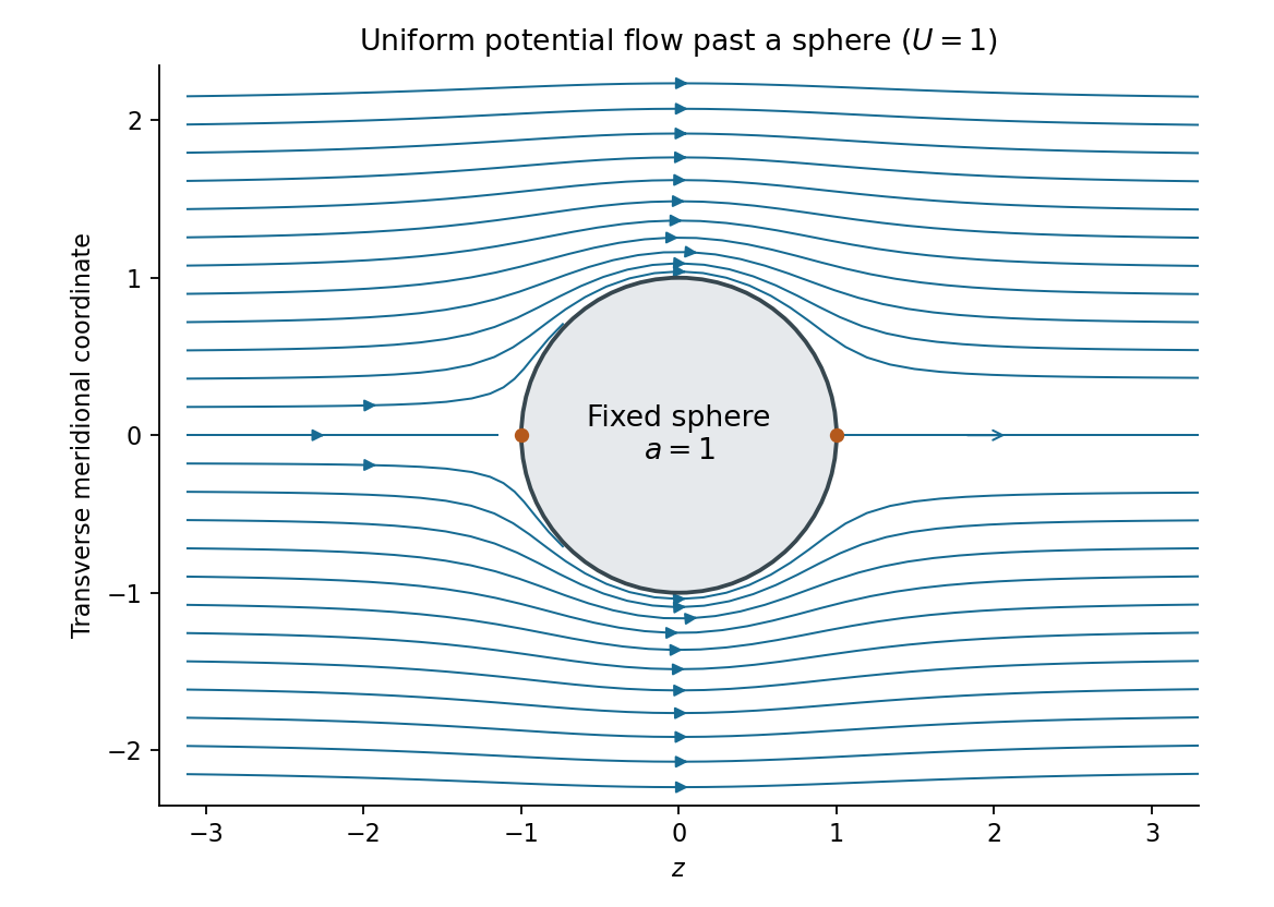
The incident uniform flow has spherical components , . Integrating the Stokes streamfunction formulas, with the additive constant chosen to vanish on the axis, givesIt is regular at the origin. Applying the sphere theorem for a Stokes streamfunction yieldsThe resulting velocity components areTo find the velocity potential, integrate and verify . This givesThe first term is the incident uniform flow, and the second is a potential dipole located inside the excluded sphere. At , the radial velocity vanishes, while the far-field velocity tends to . The poles are stagnation points; the surface tangential speed reaches at the equator. These formulas describe uniform potential flow around a fixed sphere.

Orient counterclockwise around the body. For an arc element , the body-outward unit normal vector obeys . The pressure acts normally into the body, so its force per unit length in the suppressed third direction isIntegrating givesTaking positive torque to mean counterclockwise about the origin, the infinitesimal moment is . HenceAll three expressions are per unit span. They are the normal-pressure contributions assumed by the inviscid model; a viscous traction would require extra terms. A constant pressure contributes zero net force and torque on a closed body, since .
Use the complex velocity . For this steady, constant-mass density, irrotational flow with no body force, the applicable Bernoulli equation iswith a single constant throughout the connected regular fluid region. The body's impermeability makes the velocity tangent to . Thus is real there, givingThe complex force from part (a) iswhere the constant- term vanishes. This proves the Blasius force theorem:For the moment, observe thatTherefore . The constant pressure contribution has zero real part, because . Substituting Bernoulli's principle and the same tangency identity gives the Blasius moment theorem:The real-part operation is essential: itself need not vanish, but its real part does.
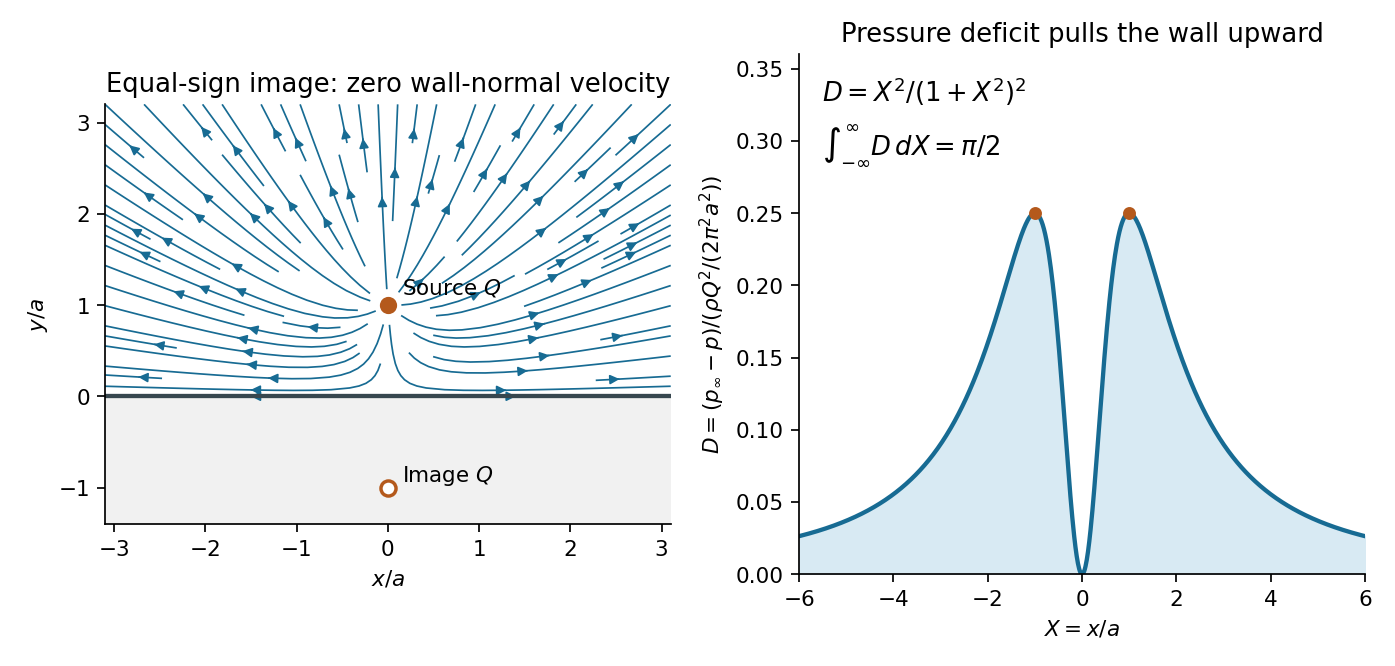
The method of images places an equal line source at , outside the physical upper half-plane. A convenient complex potential of a two-dimensional potential flow isThe two logarithms can be combined locally as ; their branches of the complex logarithm affect only the potential convention, not the single-valued complex velocity. The point source in this two-dimensional problem has the line source normalization: its outward volume flux is per unit span.
Writing , , and using , the velocity field isOn the wall , the vertical components cancel:This is the required no-penetration boundary condition. Tangential slip is permitted. At large distance the velocity decays as , and near its singular part is exactly that of the specified source; the reflected source is regular throughout the fluid. Away from the injection point, this is an incompressible flow and an irrotational flow.
Since the velocity tends to zero at infinity, the steady Bernoulli equation gives . On the wall, therefore,Compute the finite source-induced force relative to uniform ambient pressure, or equivalently use the gauge pressure . The fluid lies above the wall, so its normal force on the wall points in for positive pressure. The negative excess pressure found here consequently produces an upward net force, toward the source.
For the symmetric section , there is no horizontal force, and the vertical excess force isHere an antiderivative of is . Taking gives the hydrodynamic attraction of a wall to a line source:Each component is a force per unit length of the wall in the out-of-plane direction. The result is an attraction even though the source sends fluid away from itself: faster tangential motion reduces the wall pressure.
The excess torque about the origin isfor every , because the integrand is odd. Thus the symmetric infinite-wall limit isThe symmetric prescription matters: the separate one-sided moment integrals grow logarithmically, whereas the force integral converges absolutely. This is the appropriate Cauchy principal value for the infinite wall. If one instead asks for the absolute fluid force with no balancing ambient pressure on the other side, its vertical component on a finite section is and has no finite infinite-wall limit. The finite answer above is the flow-induced load.

Let be any material volume, moving with the velocity field . The Reynolds transport theorem in the required form isapplied componentwise when is vector-valued. Mass conservation givesSince the material volume is arbitrary, the local continuity equation follows:For an inviscid fluid with no body force, the balance of linear momentum equates the rate of change of total momentum to the boundary pressure force:using the divergence theorem. The integrand on the left expands asThe bracket vanishes by mass conservation, leaving the Euler momentum equationUnlike the incompressible flow case, the mass density need not be constant along a fluid element.
The rest state is , , . At linear order in the perturbations, the continuity equation, Euler momentum equation and the given equation of state becomeFor the acoustic component take . This is consistent with initially zero vorticity, since taking the curl of the linear momentum equation gives . Any pre-existing linear vortical component is time independent and is separate from the potential oscillations being sought.
Spatial integration of gives . Adding a function of time to the velocity potential removes without altering the velocity field. HenceSubstitute the first relation into mass conservation:Thus the velocity potential satisfies the wave equationDifferentiating that equation in time and using the same density-potential relation givesAlternatively, differentiate the linear continuity equation in time and take the divergence of the linear momentum equation. The coefficient is the sound speed, since .
The fixed upper and lower walls have zero normal velocity. Since , their no-penetration boundary conditions areFor the moving end wall, use its level-set equation . The kinematic boundary condition gives the exact impermeability relationBoth and are first order, so their product is second order. A Taylor expansion from to changes the first-order perturbation velocity only at second order as well. ThusAt infinity, select a bounded response with no waves incident from . A propagating acoustic waveguide mode must satisfy the outgoing radiation condition for a waveguide mode, while a nonpropagating mode must decay. For a time dependence , a propagating axial factor has the form , , and obeys . An evanescent factor is , .
Requiring for all frequencies would incorrectly exclude the radiated traveling waves. In this lossless channel they retain finite amplitude arbitrarily far downstream.
Let . The end-wall forcing has transverse factor , which already satisfies both fixed-wall Neumann boundary conditions. By linearity and separation of variables, seek its periodic response asSubstitution into the wave equation and the moving-wall condition givesThe acoustic waveguide cutoff is thereforeIt is the lowest nonzero transverse-mode frequency. The uniform transverse mode has no cutoff, but is not excited here because .
For , put . The axial equation has solutions . Boundedness removes the growing exponential, and fixes the coefficient. ThusThis evanescent wave oscillates in time but decays with penetration length . Its axial velocity is proportional to , while its excess pressure is proportional to . They are in phase quadrature, so their mean product, the axial acoustic energy flux, is zero.
For , put . The axial solutions are . The outgoing condition selects for the chosen time convention, andTaking the real part givesIts axial velocity is , so the moving-wall condition is satisfied with the correct sign. This is a traveling acoustic waveguide mode carrying energy toward positive . Its dispersion relation isThe larger axial phase velocity does not imply faster energy transport: the group velocity controls that transport.
At , the axial equation becomes . The imposed nonzero derivative forces a constant, which is unbounded. Thus there is no bounded periodic response at exact cutoff for this infinite, undamped, velocity-driven model. The divergent coefficients as or also show why the assumed small perturbations fail sufficiently close to cutoff at fixed forcing. Initial conditions can add free transients; the displayed formulas give the selected periodic forced response.
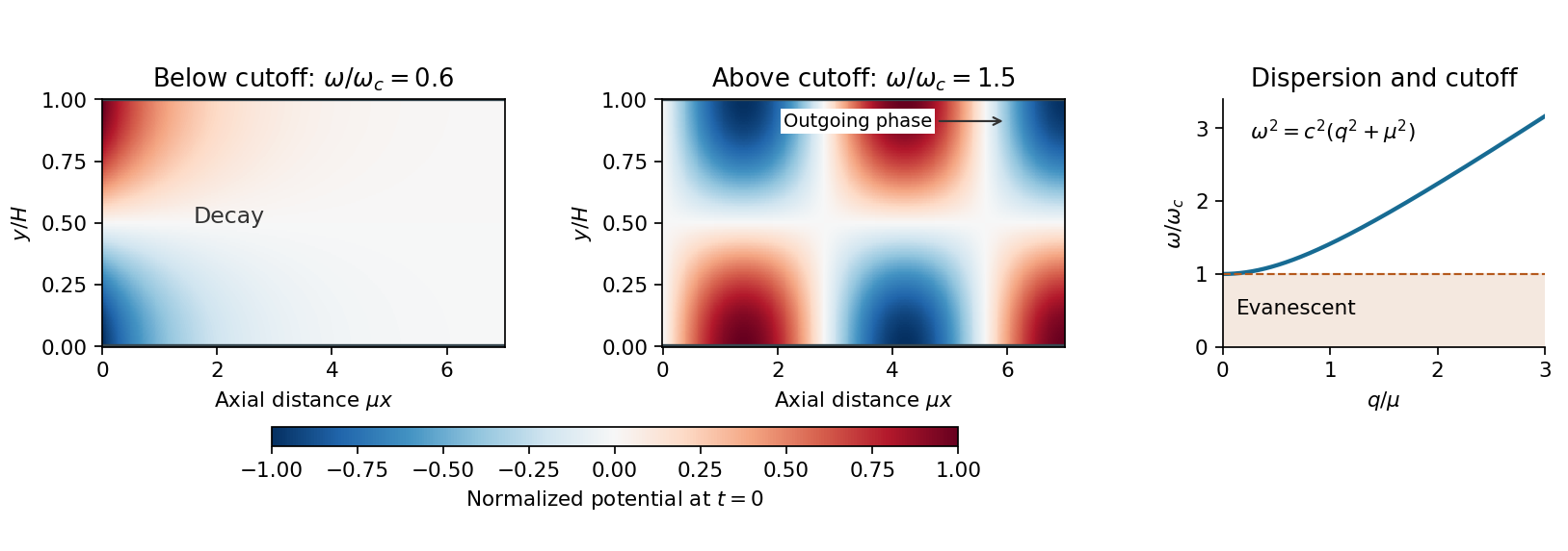
An oscillating end wall excites either an evanescent disturbance or an outgoing acoustic wave
. The transverse shape is . Below cutoff, the normalized axial potential decays exponentially; above cutoff it oscillates downstream with an outgoing phase. The right panel shows the common cutoff and the propagating dispersion branch. Details.
Articles by others on the same topic
There are currently no matching articles.