Solutions to all three questions of the University of Oxford Part A fluids and waves paper, sat on 16 June 2023. Source: original released PDF, bundle pages 242–245; paper pages 1–4. Question statements are omitted. Throughout, the liquid has constant positive mass density ; a nonzero doublet and positive bending stiffness are understood in the corresponding questions.
An irrotational flow has . Hence a velocity potential exists locally, and globally on a simply connected domain, with . The exterior of a sphere in three dimensions has this property. Constant mass density reduces the continuity equation to , soThus the velocity potential is a harmonic function. For the Euler equations, use the vorticity cross-product identityThe last term vanishes. Since , the Euler momentum equation becomesOn each connected fluid region, a function with zero gradient is spatially constant. Therefore the Unsteady Bernoulli equation isThe freedom to add a function of time to the velocity potential changes but leaves the velocity field unchanged. On a multiply connected region, zero vorticity alone guarantees only local potentials; a global single-valued velocity potential additionally requires zero circulation around every closed path.
Use the spherical symmetry of the expansion, with fluid at rest at infinity and no superposed imposed flow. The radial Laplace equation givesThe moving sphere is a material boundary: its kinematic boundary condition is . Consequently , and the spherically symmetric incompressible radial flow hasEquivalently, its volumetric flow rate through any concentric sphere is , the rate of change of the enclosed volume.
Put . The partial derivative in the Unsteady Bernoulli equation is taken at fixed spatial position, soAt infinity the velocity vanishes and , giving . Substitution cancels the arbitrary and yields the pressure field of a pulsating sphere:The distinction between at fixed and the material derivative along the moving boundary is essential here.
With zero internal pressure and negligible surface tension, pressure continuity sets the liquid-side boundary value to . Evaluating the pressure field of a pulsating sphere there givesThus the Rayleigh equation for an inviscid spherical bubble, together with its initial conditions, isFor , initially , so the physically relevant branch describes Rayleigh collapse of a spherical cavity.
Write . Multiplying the radius ordinary differential equation by gives an exact derivative:The initial conditions therefore give the first integralChoose the negative square root because the cavity starts accelerating inward. It cannot turn around while , since the squared speed is then strictly positive. Separating variables, with , proves the collapse time of a spherical cavity isHenceThe improper integral is finite: its integrand behaves as near zero and as near one. The divergent inward speed as signals a singular endpoint of this ideal incompressible flow model; the finite collapse time follows within that model.
Use for the complex potential of a two-dimensional potential flow, so . The Milne-Thomson circle theorem says that if is an incident complex potential of a two-dimensional potential flow whose singularities lie outside , thenmakes a streamline. Indeed, on that circle , so is real and the stream function is constant. This imposes the no-penetration boundary condition.
For the two-dimensional potential doublet, put and , where is real. The theorem givesUp to an additive constant, this is equivalentlyThe method of images has placed the image two-dimensional potential doublet at , inside the obstacle. We use the solution with zero added circulation and no imposed far-field flow; the original doublet is the only singularity in the liquid.
The complex potential of a two-dimensional potential flow givesAt a stagnation point, . For , taking the two square-root alternatives givesThereforeThe denominators are nonzero because . Moreoverso both stagnation points satisfy . They are distinct: equality would require . Neither is a singularity of . Conversely, the numerator of is a quadratic polynomial with nonzero leading coefficient, so these are all its finite zeros. Thus there are exactly two boundary stagnation points and none in the open fluid region. If , the flow instead vanishes everywhere, which is the degenerate exception to the assertion.
For , the Blasius force theorem states that the force per unit length exerted by a steady incompressible flow and irrotational flow on an impermeable body iswhere runs counterclockwise around the body and excludes external flow singularities. The sign corresponds to the force on the body.
Let and . The complex velocity may be writtenOnly the image point lies inside the circular contour. The term has zero residue; is regular there. In the cross term, the linear term of the Taylor expansion of suppliesThe orientation factors have canceled. The residue theorem now givesSince , : the obstacle is pulled toward the doublet, independently of . This is a force per unit length perpendicular to the plane of flow.
Keep the prescribed orientation and strength fixed, and now let the doublet position be complex. The Milne-Thomson circle theorem applies instantaneously withWhen taking its spatial derivative, is a parameter. Removing the doublet's own singular term leaves the regular complex velocity at its position:Because , the stipulated image-induced motion of a planar doublet obeys , not itself. HenceIts direction is constant. Indeed is constant and, since is real, equals . Writing in polar coordinates gives the path equationwhere the quotient is used when and the branch through with is selected. It is the straight line through parallel to . An unambiguous parametrization, also covering the degenerate polar cases, isIf , the path is radial along the positive real axis, with and changing ; it cannot be represented as a single-valued . The sign of selects which direction along the line is followed. These paths apply only while the singularity remains outside the obstacle; the model prescribes no orientation evolution.
For a plane wave with amplitude , wavenumber and angular frequency , the dispersion relation specifies which frequencies the governing equations permit. A point of fixed wave phase obeys , so the phase speed isIt is the speed of individual crests. For a narrow wave packet, two nearby plane waves with differences and have a slowly varying wave envelope depending on . Taking the limit gives the group velocityThis is the envelope's propagation speed and, in the present linear lossless wave model, the energy transport speed for a narrow packet.
A dispersive wave has phase speed dependent on wavenumber, so different components can change their relative phases and alter the packet's shape. A nondispersive wave on the chosen propagation branch has constant phase speed over the relevant band:Indeed , so equality throughout a band is equivalent to constant phase speed there. Equality at an isolated wavenumber does not make the entire wave family nondispersive.
The irrotational flow has a velocity potential with . The incompressible flow satisfies , hence the interior Laplace equation isThe ice supplies a boundary load through its bending stiffness; it does not alter this interior consequence of mass conservation.
At the rigid bed, the no-penetration boundary condition givesThe displaced surface is material, so taking the material derivative of gives the exact kinematic boundary condition for a free-surface graph:With upward vertical coordinate , the gravitational potential per unit mass is . The Unsteady Bernoulli equation, evaluated on the surface with the prescribed pressure , givesHere the spatially uniform time-dependent Bernoulli term has been absorbed into the velocity potential. The pressure is measured relative to the constant exterior pressure. This dynamic boundary condition uses the specified massless bending-cover model, with no ice inertia or tension.
Linearize about the resting state , . Introduce a dimensionless small parameter and writeholding the depth, bending stiffness and variation scales fixed. Thus both boundary displacement and induced velocity are small. For any first-order derivative , a Taylor expansion at the moving surface givesThe displacement correction to the leading field is , so evaluating it on changes it only at second order. Also and . The first-order kinematic boundary condition and dynamic boundary condition are thereforeDropping the subscript, the linearized boundary condition pair isThe fixed-bed condition remains . The source's shorthand requires a length scale: for the subsequent plane wave, small surface slope and displacement small compared with depth are sufficient conditions. Small height alone, with arbitrarily rapid spatial variation or a finite background disturbance, does not justify discarding the products.
Let , with . The surface elevation is , so . Use separation of variables in the interior Laplace equation:The term is excluded by the bed no-penetration boundary condition. The linear surface kinematic boundary condition determinesAn irrelevant additive constant is omitted. At ,The linear dynamic boundary condition then reduces toConsequently the dispersion relation of a floating elastic plate with zero plate inertia isThe negative-frequency branch gives propagation in the opposite direction. For signed wavenumber, replace by in the squared-frequency formula. Setting recovers the finite-depth surface gravity wave relation, a useful sign check.
In the deep-water limit , . Put . The squared phase speed of the flexural-gravity wave is thenIt diverges as and as in this limiting model. Its unique stationary point satisfiesThe second derivative is positive. Using gives the minimum phase speed of a flexural-gravity wave:This is the deep-water minimum: applying it to a finite depth requires . Otherwise the factor must be retained in the minimization. Within the deep-water approximation, phase speed and group velocity coincide at , although the wave family remains dispersive.
Define the dimensionless parameterThe stipulated hierarchy implies both andThus the finite-depth correction uses , while the restoring effect of bending stiffness is small compared with gravity. The dispersion relation becomesHence, to leading order, these surface gravity waves are nondispersive waves withFor clarity, the first corrections to the phase speed areThey exhibit the weak residual wave dispersion at finite wavenumber. The claimed nondispersive behavior is the asymptotic leading-order result, not exact equality for the complete relation.
Solutions to all three questions of the University of Oxford Part A fluids and waves paper, sat on 24 June 2021. Source: original released PDF, bundle pages 236–238; paper pages 1–3.
The velocity of a fluid element is the time derivative of its position with its Lagrangian coordinates held fixed. Direct differentiation givesReplacing the Lagrangian coordinates by the current Eulerian coordinates therefore gives the velocity fieldThe distinction between following a fluid element and differentiating at fixed Eulerian coordinates is what connects the given deformation map to this velocity field.
For a planar incompressible flow, the divergence of the velocity field must vanish. HereEquivalently, the Jacobian determinant of the deformation map isso every material area is preserved. However, the out-of-plane vorticity isSince , this vorticity never vanishes. The motion is an incompressible flow but is not an irrotational flow; its local spin is clockwise.
Adopt the streamfunction convention , . Integrating the first component of the velocity field in gives . The second component then requires . Thus, omitting an arbitrary function of time,At a fixed instant, the streamlines are the connected curves . To classify this quadratic form, introduce the invertible scaled and rotated coordinatesThenFor , both coefficients are positive. Every therefore gives an ellipse, and is the stagnation point at the origin. For , the quadratic form is an indefinite quadratic form: each gives a hyperbola. The level consists of the straight separatriceswhose rays approach or leave the origin; the origin itself is a stagnation point. At the transition , , so the nonstationary streamlines are parallel straight lines and is a line of stagnation points. These are instantaneous streamlines; the time dependence means that they need not coincide with pathlines.
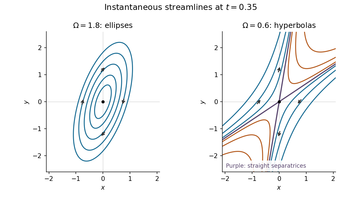
Instantaneous elliptical and hyperbolic streamlines at the same positive time
. Details. 
Use for the complex potential of a two-dimensional potential flow, so its complex velocity is . The incident uniform flow and line source haveThe coefficient of the complex logarithm is one because a line source of strength has complex potential of a two-dimensional potential flow , and here . Applying the Milne-Thomson circle theorem to the unit circle givesSince , locally consistent branches of the complex logarithm giveChanges of branch only alter the constant in a local expression; is single valued away from its singularities. The added terms represent a two-dimensional potential doublet at the origin, an image line source at , and a compensating line sink at the origin. The image line source and line sink have equal and opposite strengths, so no net volume flux enters the cylinder.
On , the Milne-Thomson circle theorem makes up to a constant. Consequently the streamfunction is constant there, establishing the no-penetration boundary condition. All line source strengths are real, and the two-dimensional potential doublet has zero circulation, so the circulation around the cylinder is zero. There is no additional line vortex term.
Let denote the force per unit length exerted by the fluid on the cylinder, and let be the constant mass density. For a counterclockwise contour around the unit circle, the Blasius force theorem givesAn efficient use of the residue theorem finds the sum of the enclosed residues by subtracting the external pole at from the sum of all finite residues. At large ,The sum of all finite residues of is therefore . At , write , with a holomorphic function near . ThenThusUsing and givesThe vanishing vertical force also follows from reflection symmetry about the real axis. This force on a unit cylinder due to a uniform flow and an external source uses the counterclockwise orientation in the Blasius force theorem to fix the sign of the horizontal force.
Since , the denominator inis positive. The positive root of isThe other root is negative, so the horizontal force points in the positive direction for , vanishes at , and points in the negative direction for . In particular, the nearby line source pulls the cylinder towards itself as , while at large the horizontal force is .
The Joukowski map is a holomorphic function for , withA holomorphic function is a local conformal map wherever its derivative is nonzero. Hence the two finite nonzero critical points areThey lie on the boundary of the fluid region. At the displayed formula has a pole and is undefined as a map to the finite complex plane; zero is outside the fluid region. Thus is locally conformal everywhere in the fluid.
For ,Both factors are positive in the fluid region, so its image is contained in the upper half-plane. The boundary correspondence is also explicit: on the upper unit semicircle, gives , while the real rays and map onto the rays and .
To prove the image is the whole upper half-plane, fix any . The equation isIts roots have product one. Neither root can have unit modulus, since that would make real. Exactly one root therefore has modulus greater than one. For that root the formula for forces , so it belongs to the fluid region. Moreover, if , thenTwo distinct roots in the fluid region would require , impossible when both moduli exceed one. Thus the Joukowski map of the upper exterior of a unit disk is a bijection from the fluid region onto the upper half-plane.
The quadratic formula gives two algebraic possibilities. To select one consistent holomorphic square root, setwhere each factor is the principal square root. Both arguments lie in the upper half-plane, so neither crosses its branch cut. This choice satisfies and at large in the upper half-plane. The required inverse function isFor , , this gives , whose modulus exceeds one. As varies continuously in the upper half-plane, this root cannot cross , since that would make real. Hence the selected root always lies in the fluid region. The other root is its reciprocal and lies inside the unit disk. Simply writing the principal square root of would not specify this branch correctly throughout the upper half-plane.
The line vortex is mapped toIts imaginary part is positive because lies in the fluid region. A conformal map preserves the circulation of the local line vortex, so its strength in the mapped complex plane is still .
Take positive to mean counterclockwise circulation. A line vortex at has complex potential of a two-dimensional potential flow . The method of images imposes the no-penetration boundary condition on the real axis by placing an image line vortex of strength at . ThusFor real , the numerator and denominator have equal modulus, so the streamfunction isThe real axis is therefore a streamline. The image line vortex lies outside the mapped fluid region, while the complex velocitydecays as . This selects the flow due to the line vortex and the boundary, without superposing an imposed background velocity field.
The physical complex potential of a two-dimensional potential flow is . Applying the chain rule gives the complex velocityThe physical velocity is . A useful equivalent expression follows fromFactoring the image expression in the same way makes the terms cancel, leavingThis represents the physical line vortex at , an image line vortex of the same strength at , and image point vortices of opposite strength at and . All three image locations are outside the fluid region. Both boundary pieces inherit the constant streamfunction of the real axis in the mapped complex plane.
A free point vortex is advected by the regular part of the velocity field at its position. Its own singular complex velocity must first be subtracted. The image expression therefore givesEquivalently, is the complex conjugate of the boxed expression. This is the instantaneous velocity, evaluated with the current value of .
To see why mapping the image velocity alone would miss a term, expand the mapped physical singularity:Thus the same point-vortex drift under a conformal map can be writtenThe finite term involving is part of the physical regular velocity field.
If with , direct substitution into the image expression givesThe bracket is strictly positive, and the result is real. Hence a positive line vortex initially moves horizontally to the right, a negative line vortex moves to the left, and the initial vertical velocity is zero. As , the leading term is the familiar drift of a point vortex above a straight wall.
For an irrotational flow, write . The incompressible flow condition then gives the Laplace equationAt leading order in a small disturbance this equation holds on . Including gravity, the Unsteady Bernoulli equation isChoose the time-dependent additive freedom in the velocity potential so that . Neglecting surface tension, pressure continuity at the free surface gives the exact dynamic conditionThe free surface is a material boundary: applying the material derivative to yields the kinematic boundary condition for a free-surface graphFor a small disturbance, the Taylor expansion from to changes the first-order velocity potential and its partial derivatives only at second order. Both and are also second-order terms. The linearized free-surface boundary conditions are thereforeThe fixed bed has the no-penetration boundary conditionThe required approximation is small surface elevation, small wave steepness, and small velocity perturbations. The stated alone does not ensure this approximation near resonance.
Seek the travelling forced component of the surface elevation in the form , where and is a signed coefficient. The forcing has wavenumber one. Separation of variables in the Laplace equation, followed by the bed no-penetration boundary condition, givesSince , the surface kinematic boundary condition requires , soAt , . The dynamic member of the linearized free-surface boundary conditions therefore becomesConsequently the signed response and the nonnegative amplitude areThe travelling-pressure response of finite-depth surface gravity waves is opposite in phase to the imposed pressure below the resonant speed and in phase above it. These expressions describe the travelling forced component; freely propagating surface gravity waves can be superposed to meet additional initial conditions.
The denominator of the travelling response vanishes atFor the positive speeds in the paper, a finite travelling response exists whenever . At , the dynamic condition would reduce to , which is impossible. The finite-depth dispersion relation of a surface gravity wave with wavenumber is . At , its phase speed equals : the moving pressure pattern drives a natural surface gravity wave at its own speed, producing resonance.
The restriction concerns a bounded travelling response. To distinguish this from existence of a solution of an initial value problem, set , , and . Ifthe linearized free-surface boundary conditions reduce to the forced harmonic oscillatorFor example, if the forcing is switched on at from a flat surface with zero initial velocity, then, for ,This satisfies and contains both free oscillations and the forced component. At a solution of the initial value problem still exists, but its particular solution containswhich grows linearly with time. Thus the ideal inviscid flow model predicts resonant growth rather than a finite constant amplitude. Additional free oscillations can set the initial conditions but cannot remove that secular growth.
For , the nonnegative amplitude isIts first two derivatives are positive in this interval:The graph is increasing and convex, starts with a horizontal tangent at the limiting value , and has a vertical asymptote at . Therefore the hydrostatic lower bound for a travelling-pressure response isBecause the paper assumes , this is an infimum, approached as , rather than an attained minimum. If the stationary limit is admitted, equality holds: the hydrostatic equilibrium condition is . Near resonance,The divergence describes the linear model; sufficiently close to the small-disturbance assumptions fail. The lower bound and sketch refer to the travelling forced component, since adding free oscillations can change the instantaneous surface elevation.
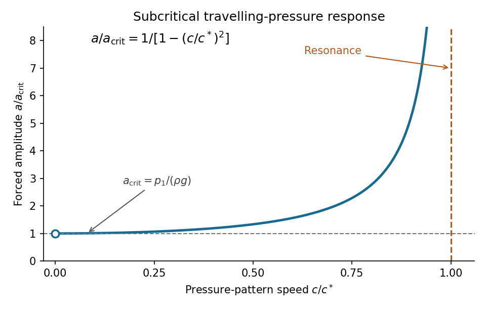
Subcritical travelling-wave amplitude rises from its hydrostatic lower bound and diverges at resonance
. Details. 
Articles by others on the same topic
There are currently no matching articles.